Mystics & Statistics

A blog on quantitative historical analysis hosted by The Dupuy Institute

Wargaming Multi-Domain Battle: The Base Of Sand Problem

“JTLS Overview Movie by Rolands & Associates” [YouTube]

[This piece was originally posted on 10 April 2017.]

As the U.S. Army and U.S. Marine Corps work together to develop their joint Multi-Domain Battle concept, wargaming and simulation will play a significant role. Aspects of the construct have already been explored through the Army’s Unified Challenge, Joint Warfighting Assessment, and Austere Challenge exercises, and upcoming Unified Quest and U.S. Army, Pacific war games and exercises. U.S. Pacific Command and U.S. European Command also have simulations and exercises scheduled.

A great deal of importance has been placed on the knowledge derived from these activities. As the U.S. Army Training and Doctrine Command recently stated,

Concept analysis informed by joint and multinational learning events…will yield the capabilities required of multi-domain battle. Resulting doctrine, organization, training, materiel, leadership, personnel and facilities solutions will increase the capacity and capability of the future force while incorporating new formations and organizations.

There is, however, a problem afflicting the Defense Department’s wargames, of which the military operations research and models and simulations communities have long been aware, but have been slow to address: their models are built on a thin foundation of empirical knowledge about the phenomenon of combat. None have proven the ability to replicate real-world battle experience. This is known as the “base of sand” problem.

A Brief History of The Base of Sand

All combat models and simulations are abstracted theories of how combat works. Combat modeling in the United States began in the early 1950s as an extension of military operations research that began during World War II. Early model designers did not have large base of empirical combat data from which to derive their models. Although a start had been made during World War II and the Korean War to collect real-world battlefield data from observation and military unit records, an effort that provided useful initial insights, no systematic effort has ever been made to identify and assemble such information. In the absence of extensive empirical combat data, model designers turned instead to concepts of combat drawn from official military doctrine (usually of uncertain provenance), subject matter expertise, historians and theorists, the physical sciences, or their own best guesses.

As the U.S. government’s interest in scientific management methods blossomed in the late 1950s and 1960s, the Defense Department’s support for operations research and use of combat modeling in planning and analysis grew as well. By the early 1970s, it became evident that basic research on combat had not kept pace. A survey of existing combat models by Gary Shubik and Martin Brewer for RAND in 1972 concluded that

Basic research and knowledge is lacking. The majority of the MSGs [models, simulations and games] sampled are living off a very slender intellectual investment in fundamental knowledge…. [T]he need for basic research is so critical that if no other funding were available we would favor a plan to reduce by a significant proportion all current expenditures for MSGs and to use the saving for basic research.

In 1975, John Stockfish took a direct look at the use of data and combat models for managing decisions regarding conventional military forces for RAND. He emphatically stated that “[T]he need for better and more empirical work, including operational testing, is of such a magnitude that a major reallocating of talent from model building to fundamental empirical work is called for.”

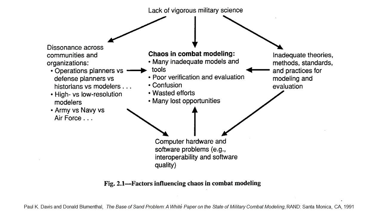
In 1991, Paul K. Davis, an analyst for RAND, and Donald Blumenthal, a consultant to the Livermore National Laboratory, published an assessment of the state of Defense Department combat modeling. It began as a discussion between senior scientists and analysts from RAND, Livermore, and the NASA Jet Propulsion Laboratory, and the Defense Advanced Research Projects Agency (DARPA) sponsored an ensuing report, The Base of Sand Problem: A White Paper on the State of Military Combat Modeling.

Davis and Blumenthal contended

The [Defense Department] is becoming critically dependent on combat models (including simulations and war games)—even more dependent than in the past. There is considerable activity to improve model interoperability and capabilities for distributed war gaming. In contrast to this interest in model-related technology, there has been far too little interest in the substance of the models and the validity of the lessons learned from using them. In our view, the DoD does not appreciate that in many cases the models are built on a base of sand…

[T]he DoD’s approach in developing and using combat models, including simulations and war games, is fatally flawed—so flawed that it cannot be corrected with anything less than structural changes in management and concept. [Original emphasis]

As a remedy, the authors recommended that the Defense Department create an office to stimulate a national military science program. This Office of Military Science would promote and sponsor basic research on war and warfare while still relying on the military services and other agencies for most research and analysis.

Davis and Blumenthal initially drafted their white paper before the 1991 Gulf War, but the performance of the Defense Department’s models and simulations in that conflict underscored the very problems they described. Defense Department wargames during initial planning for the conflict reportedly predicted tens of thousands of U.S. combat casualties. These simulations were said to have led to major changes in U.S. Central Command’s operational plan. When the casualty estimates leaked, they caused great public consternation and inevitable Congressional hearings.

While all pre-conflict estimates of U.S. casualties in the Gulf War turned out to be too high, the Defense Department’s predictions were the most inaccurate, by several orders of magnitude. This performance, along with Davis and Blumenthal’s scathing critique, should have called the Defense Department’s entire modeling and simulation effort into question. But it did not.

The Problem Persists

The Defense Department’s current generation of models and simulations harbor the same weaknesses as the ones in use in the 1990s. Some are new iterations of old models with updated graphics and code, but using the same theoretical assumptions about combat. In most cases, no one other than the designers knows exactly what data and concepts the models are based upon. This practice is known in the technology world as black boxing. While black boxing may be an essential business practice in the competitive world of government consulting, it makes independently evaluating the validity of combat models and simulations nearly impossible. This should be of major concern because many models and simulations in use today contain known flaws.

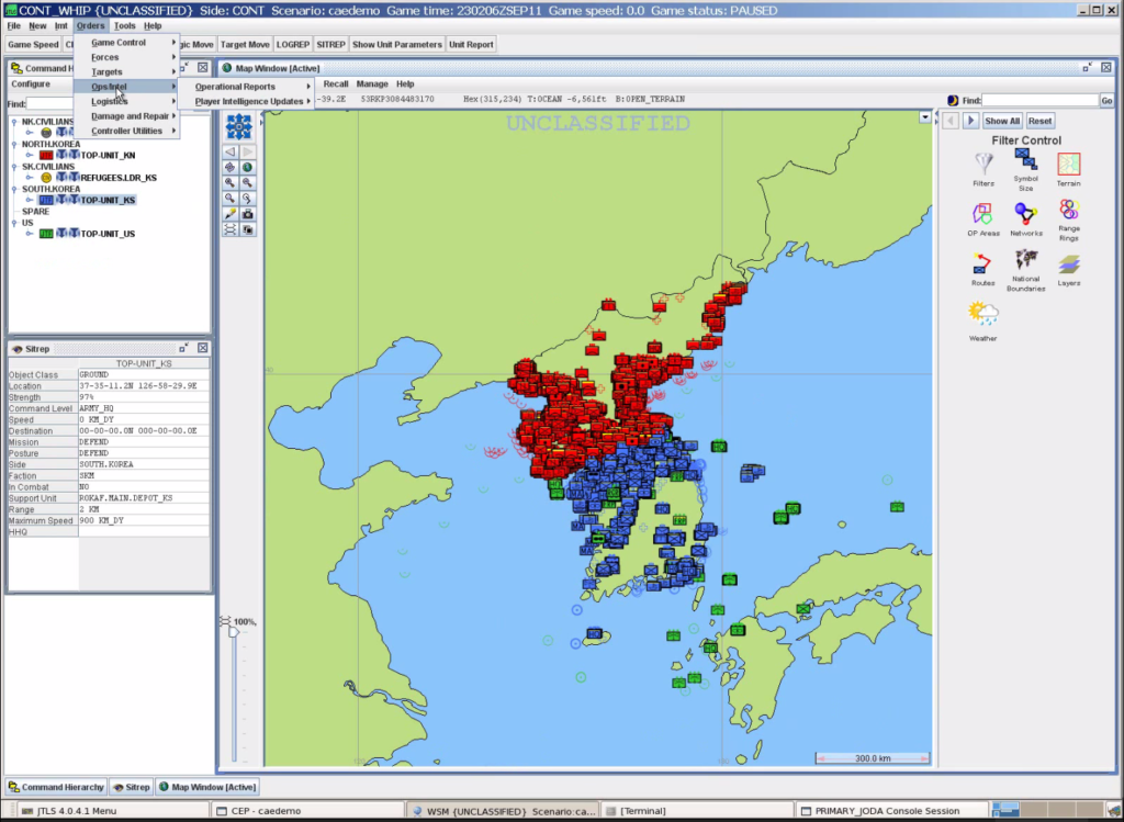
Some, such as  Joint Theater Level Simulation (JTLS), use the Lanchester equations for calculating attrition in ground combat. However, multiple studies have shown that these equations are incapable of replicating real-world combat. British engineer Frederick W. Lanchester developed and published them in 1916 as an abstract conceptualization of aerial combat, stating himself that he did not believe they were applicable to ground combat. If Lanchester-based models cannot accurately represent historical combat, how can there be any confidence that they are realistically predicting future combat?

Others, such as the Joint Conflict And Tactical Simulation (JCATS), MAGTF Tactical Warfare System (MTWS), and Warfighters’ Simulation (WARSIM) adjudicate ground combat using probability of hit/probability of kill (pH/pK) algorithms. Corps Battle Simulation (CBS) uses pH/pK for direct fire attrition and a modified version of Lanchester for indirect fire. While these probabilities are developed from real-world weapon system proving ground data, their application in the models is combined with inputs from subjective sources, such as outputs from other combat models, which are likely not based on real-world data. Multiplying an empirically-derived figure by a judgement-based coefficient results in a judgement-based estimate, which might be accurate or it might not. No one really knows.

Potential Remedies

One way of assessing the accuracy of these models and simulations would be to test them against real-world combat data, which does exist. In theory, Defense Department models and simulations are supposed to be subjected to validation, verification, and accreditation, but in reality this is seldom, if ever, rigorously done. Combat modelers could also open the underlying theories and data behind their models and simulations for peer review.

The problem is not confined to government-sponsored research and development. In his award-winning 2004 book examining the bases for victory and defeat in battle, Military Power: Explaining Victory and Defeat in Modern Battle, analyst Stephen Biddle noted that the study of military science had been neglected in the academic world as well. “[F]or at least a generation, the study of war’s conduct has fallen between the stools of the institutional structure of modern academia and government,” he wrote.

This state of affairs seems remarkable given the enormous stakes that are being placed on the output of the Defense Department’s modeling and simulation activities. After decades of neglect, remedying this would require a dedicated commitment to sustained basic research on the military science of combat and warfare, with no promise of a tangible short-term return on investment. Yet, as Biddle pointed out, “With so much at stake, we surely must do better.”

[NOTE: The attrition methodologies used in CBS and WARSIM have been corrected since this post was originally published per comments provided by their developers.]

A Force Ratio Model Applied to Afghanistan

As many people are aware, the one logit regression that we had confidence in from the 83 insurgency cases we tested was a force ratio versus outcome model. This is discussed in the following blog post and in Chapter 6 of my book America’s Modern Wars.

We probably need to keep talking about Afghanistan

The key was that we ended up with two very different curves: one if the insurgency was based upon a central idea (like nationalism) and a lesser curve if the insurgency was based upon limited political concept (a regional or factional insurgency). Now, we never really determined which applied to Afghanistan, because we actually never had a contract to do any work or analysis on Afghanistan. I am hesitant to reach conclusions without some research.

But let us look at the force ratios there now. I estimate that the insurgency has at least 60,000 full-time and part-time insurgents. There may have more than that. But, working backwards from the incident count of 20,000+ a year, and comparing those incident counts with insurgent strengths in past insurgencies, leads me to conclude that it is at least 60,000 insurgents. This process is discussed in depth in Chapter 11 of my book. Let’s work with that figure for a moment.

The counterinsurgent forces consist of supposedly almost 400,000 people. Except…in our model we only counted army and air force, and only counted police only if it was clear that counterinsurgent operations was their primary duty. Therefore our model did not count most police.

Parsing out the data in Wikipedia shows that the Afghan Army and Air Force total around 195,000 active in 2014. The Wikipedia source was this article: https://www.pajhwok.com/en/2015/03/10/mohammadi-asks-troops-stand-united. I have no idea how correct this number is. It might be a little optimistic (see my comments about auditing the police force rolls).

The Afghan National Police (ANP) have 157,000 members in September 2013 (again Wikipedia). I note that the UNAMA report in December 2018 on the audit reduced the ANP payroll from 147,875 to 106,189. But, this is a national police force. It includes uniformed police, border police, a criminal investigation division of 4,148 investigators, etc. Let’s say for convenience that half of them are doing traditional police work and half are doing counterinsurgent work. I have no idea if this is a good or reasonable split. So let’s say 53,000 ANP police involved in the counterinsurgency effort. The Afghan Local Police (ALP) are 19,600 as of February 2013. As they are clearly part of the counterinsurgency effort, I will count them.

The 18,000 ISAF are mostly training, so I am not sure how they should be counted, but we will count them. No sure if we should count the 20,000 contractors, as quite simply, there were not a lot of contractors in our previous 83 cases. The use of private contractors to fight insurgencies is a relatively new approach. For now I will not count them.

So, let’s count counterinsurgent strength at 195,000 + 53,000 ANP + 19,600 ALP + 18,000 ISAF. This gives a counterinsurgent strength of 285,600 compared to an insurgent strength of 60,000. This is a 4.76-to-1 force ratio. This is a very precise number created from some very fuzzy data.

Now, if I look at the curve for an insurgency based upon an limited political concept, and I see that an 4.76-to-1 force ratio means that the counterinsurgent won roughly 86% of the time (see page 65 of my book). This is favorable. But right now, it doesn’t really look like we have been winning in Afghanistan over the last eight years.

On the other hand, if I code this as an insurgency based upon a central idea I see that a 4.76-to-1 force ratio results in the counterinsurgent winning 19% of the time. This is much worse.

So…I have yet to make a determination as to which curve should apply in this case. Perhaps neither do, as Afghanistan is a unique and complex case. Properly analyzing this would require a level-of-effort beyond what I am willing to invest. Keep in mind that our Iraq estimate was funded in 2004 (see Chapter 1 of my book). It was also ignored.

Some Statistics on Afghanistan (Jan 2019)

Camp Lonestar, near Jalabad, 7 October 2010 (Photo by William A. Lawrence II)

The fighting in Afghanistan continues, with a major attack reported a day ago in west Afghanistan that resulted in the death of 21 police and militia and 9 wounded: https://www.usnews.com/news/world/articles/2019-01-07/taliban-storm-security-posts-in-west-afghanistan-kill-21. This was a pretty significant fight, with the government claiming 15 Taliban militants killed and 10 wounded.

I do lean on the Secretary General reports quarterly reports on Afghanistan for my data, as it may be the most trusted source available. Those reports are here:

https://unama.unmissions.org/secretary-general-reports

So what are the current statistics?:

              Security           Incidences      Civilian

Year      Incidences       Per Month       Deaths

2008        8,893                  741

2009      11,524                  960

2010      19,403               1,617

2011      22,903               1,909

2012      18,441?             1,537?                             *

2013      20,093               1,674               2,959

2014      22,051               1,838               3,699

2015      22,634               1,886               3,545

2016      23,712               1,976               3,498

2017      23,744               1,979               3,438

2018      22,745               1,895               3,731      Estimated (see below)


At the start of 2013, we still had 66,000 troops in Afghanistan, although we were drawing them down. There were 251 U.S. troops killed in 2012 (310 killed from all causes) and 85 in 2013 (127 killed from all causes). Over the course of 2013, 34,000 troops were to be withdrawn and the U.S. involvement to end sometime in 2015. We did withdrawn the troops, but really have not ended our involvement. According to Wikipeida we have 18,000+ ISAF forces there (mostly American) and 20,000+ contractors. I have not checked these figures. The latest reports I have seen say around 14,000 American troops in Afghanistan. The Afghans have over 300,000 security forces (Army, Air Force, National Police, Local Police, etc.) to conduct the counterinsurgency.

The Secretary General 7 December 2018 report does note that “On 30 August, the Government complete the personnel asset inventory for existing Afghan National Police personnel…..Out of 147,875 records, 106,189 personnel were identified as legitimate for the payment of salaries. The remaining 41,686 records were removed from the payroll for such reasons as retirement, desertion and attrition.”

As we note in Chapter Twenty-One of my book America’s Modern Wars: “The 2013 figure of 20,093 incidents a year does argue for a significant insurgency force. If we use a conservative figure of 333 incidents per thousand insurgents, then we are looking at more than 60,000 full-time and part-time insurgents.”

This war does appear to be flat-lined, with no end in sight.


Camp Lonestar, near Jalabad, 7 October 2010 (Photo by William A. Lawrence II)

————————————————————————————————————-

Notes for 2018 estimates:

  1. 15 December 2017-15 February 2018: 3,521 security incidences (6% decrease from previous year).

  2. 15 February-15 May: 5,675 security incidences (7% decrease from previous year).

  3. 15 May – 15 August: 5,800 security incidences (10% decrease from previous year)

  4. 16 August – 15 November: 5,854 security incidences (2% decrease from previous year)
  5. 1 January – 30 September: 2,798 civilian deaths (highest number since 2014)

    1. UNAMA attributed 65% of all civilian casualties to anti-government elements
      1.  35% to Taliban
      2.  25% to ISIL-KP
      3. 5% other
    2. 22% to pro-government forces
      1. 16% to Afghan national security forces
      2. 5% to international military forces
      3. 1% to pro-government armed groups
    3. 10% unattributed crossfire during ground engagements
    4. 3% to other incidents, including explosive remnants of war and cross-border shelling
    5. Causes of civilian deaths
      1. 45% caused by improvised explosive devices.
      2. 29% caused by ground engagements
        1. More than half of those casualties (313 people killed and 336 injured) caused by aerial strikes by pro-government forces)

 * The 2012 stats are a little garbled. They are missing 1-15 August 2012, but include 1 January through 15 February 2013.

TDI Friday Read: Multi-Domain Battle/Operations Doctrine

With the December 2018 update of the U.S. Army’s Multi-Domain Operations (MDO) concept, this seems like a good time to review the evolution of doctrinal thinking about it. We will start with the event that sparked the Army’s thinking about the subject: the 2014 rocket artillery barrage fired from Russian territory that devastated Ukrainian Army forces near the village of Zelenopillya. From there we will look at the evolution of Army thinking beginning with the initial draft of an operating concept for Multi-Domain Battle (MDB) in 2017. To conclude, we will re-up two articles expressing misgivings over the manner with which these doctrinal concepts are being developed, and the direction they are taking.

The Russian Artillery Strike That Spooked The U.S. Army

Army And Marine Corps Join Forces To Define Multi-Domain Battle Concept

Army/Marine Multi-Domain Battle White Paper Available

What Would An Army Optimized For Multi-Domain Battle Look Like?

Sketching Out Multi-Domain Battle Operational Doctrine

U.S. Army Updates Draft Multi-Domain Battle Operating Concept

U.S. Army Multi-Domain Operations Concept Continues Evolving

U.S. Army Doctrine and Future Warfare


Quantifying the Holocaust

Odilo Globocnik, SS and Police Leader in the Lublin district of the General Government territory in German-occupied Poland, was placed in charge of Operation Reinhardt by SS Reichsführer Heinrich Himmler. [Wikipedia]

The devastation and horror of the Holocaust makes it difficult to truly wrap one’s head around its immense scale. Six million murdered Jews is a number so large that it is hard to comprehend, much less understand in detail. While there are many accounts of individual experiences, the wholesale destruction of the Nazi German documentation of their genocide has made it difficult to gauge the dynamics of their activities.

However, in a new study, Lewi Stone, Professor of Biomathematics at RMIT University in Australia, has used an obscure railroad dataset to reconstruct the size and scale of a specific action by the Germans in eastern Poland and western Ukraine in 1942. “Quantifying the Holocaust: Hyperintense kill rates during the Nazi genocide,” (Not paywalled. Yet.) published on 2 January in the journal Science Advances, uses train schedule data published in 1987 by historian Yitzhak Arad to track the geographical and temporal dimensions of some 1.7 Jews transported to the Treblinka, Belzec and Sobibor death camps in the late summer and early autumn of 1942.

This action, known as Operation Reinhardt, originated during the Wansee Conference in January 1942 as the plan to carry out Hitler’s Final Solution to exterminate Europe’s Jews. In July, Hitler “ordered all action speeded up” which led to a frenzy of roundups by SS (Schutzstaffel) groups from over 400 Jewish communities in Poland and Ukraine, and transport via 500 trains to the three camps along the Polish-Soviet border. In just 100 days, 1.7 million people had been relocated and almost 1.5 million of them were murdered (“special treatment” (Sonderbehandlung)), most upon arrival at the camps. This phase of Reinhardt came to an end in November 1942 because the Nazis had run out of people to kill.

This three-month period was by far the most intensely murderous phase of the Holocaust, carried out simultaneously with the German summer military offensive that culminated in disastrous battlefield defeat at the hands of the Soviets at Stalingrad at year’s end. 500,000 Jews were killed per month, or an average of 15,000 per day. Even parsed from the overall totals, these numbers remain hard to grasp.

Stone’s research is innovative and sobering. His article can currently be downloaded in PDF format. His piece in The Conversation includes interactive online charts. He also produced a video the presents his findings chronologically and spatially:

Panzer Battalions in LSSAH in July 1943 – II

This is a follow-up to this posting:

Panzer Battalions in LSSAH in July 1943

The LSSAH Panzer Grenadier Division usually had two panzer battalions. Before July the I Panzer Battalion had been sent back to Germany to arm up with Panther tanks. This had lead some authors to conclude that in July 1943, the LSSAH had only the II Panzer Battalion. Yet the unit’s tank strength is so high that this is hard to justify. Either the LSSAH Division in July 1943 had:

  1. Over-strength tank companies
  2. A 4th company in the II Panzer Battalion
  3. A temporary I Panzer Battalion

I have found nothing in the last four months to establish with certainly what was the case, but additional evidence does indicate that they had a temporary I Panzer Battalion.

The first piece of evidence is drawn from a division history book, called Liebstandarte III, by Rudolf Lehmann, who was the chief of staff of the Panzer Regiment. It states that they had around 33 tanks at hill 252.2 on the afternoon or evening of the 11th. It has been reported that the entire II Panzer Battalion moved up there on the 11th, and then pulled back their 5th and 7th companies, leaving the 6th company in the area of hill 252.2. The 6th Panzer Company was reported to have only 7 tanks operational on the morning of the 12th. So, II Panzer Battalion may have had three companies of 7-12 tanks each, and the battalion staff, and maybe some or all of the regimental staff there. The LSSAH Division according to the Kursk Data Base had as of the end of the day on 11 July 1943: 2 Panzer Is, 4 Panzer IIs, 1 Panzer III short, 4 Panzer III longs, 7 Panzer III Command tanks, 47 Panzer IV longs and 4 Panzer VIs for a total of 69 tanks in the panzer regiment. Ignoring the 4 Tiger tanks, this leaves 32 tanks unaccounted for. This could well be the complement of a temporary I Panzer Battalion.

The second unresolved issue is that the Soviet XVIIII Tank Corps is reported to have encountered dug-in tanks as they tried to push beyond Vasilyevka along the Psel River. They reported that their advance was halted by tank fire from the western outskirts of Vasilyevka. They also report at 1400 (Moscow time) repulsing a German counterattack by 50 tanks from the Bogoroditskoye area (just west of Vasilyevka, south of the Psel).

With the II Panzer Battalion being opposite the XXIX Tank Corps, then one wonders who and where those “dug-in tanks” were from. It is reported in some sources that the Tiger company, which was in the rear when the fighting started, moved to the left flank, but most likely there was another tank formation there. If the II Panzer Battalion was covering the right half of the LSSAH’s front, then it would appear that the rest of the front would have been covered by a temporary I Panzer Battalion of at least three companies.

This leads to me lean even more so to the conclusion that the LSSAH had a temporary I Panzer Battalion of at least three companies, the II Panzer Battalion of three companies, and the Tiger company, which was assigned to the II Panzer Battalion.

Force Draw Downs

I do discuss force draw downs in my book America’s Modern Wars: Understanding Iraq, Afghanistan and Vietnam. It is in Chapter 19 called “Withdrawal and War Termination” (pages 237-242). To quote from parts of that chapter:

The missing piece of analysis in both our work and in that of many of the various counterinsurgent theorists is how does one terminate or end these wars, and what is the best way to do so? This is not an insignificant point. We did propose doing exactly such a study in several of our reports, briefings and conversations, but no one expressed a strong interest in examining war termination…..

In our initial look at 28 cases, we found only three cases where the counterinsurgents were able to reduce or choose to significantly reduce force strength during the course of an insurgency. These are Malaya, Northern Ireland and Vietnam. With our expanded database of 83 cases, these are still the only three cases of such.

Let us look at each in turn. The case of Malaya is illustrated below:

The most intense phase of the insurgency was from 1958 to 1952. Peak counterinsurgent deaths were 488 in 1951, with 272 in 1952 and only 95 in 1953. Over the course of 1959 and 1960, there were only three deaths.

When one looks at counterinsurgent force strength over that period, one notes a large decline in strength, but in fact, it is a decline in militia strength. Commonwealth troop strength peaked at 29,656 in 1956, consisting of UK troops, Gurkhas and Australians. It declined to 16,939 in 1960. Basically, even with no combat occurring for two years, the troop strength of the intervening forces (“UK Combat Troops” on the first graph) was reduced by one half and only during last couple of years. The decline is Malayan strength is primarily due to police force declining after 1953 and the “Special Constabulary” declining after 1952 and eventually being reduced to zero. There was also a Malayan Home Guard that was briefly up to 300,000 people, but most of them were never armed and were eventually disbanded.

This is the best case we have of a force draw down, and it was only done to any significance late in the war, where the insurgency was pretty much reduced to 400 or so fighters sitting across the narrow border with Thailand and scattered remnants being policed inside of Malaya.

Northern Ireland is another case in which the degree of activity was very intense early on. For example:

On the other hand, force strength does not draw down much.

In this case the peak counterinsurgent strength was 48,341 in 1972, and the counterinsurgent strength is still 22,691 in 2002. These two cases show the limitation of a draw down.

In the case of Vietnam, there was a four-year-long massive build up, and then four years of equally hasty withdrawal. This is clearly not the way to conduct a war and is discussed in more depth in Chapter Twenty-Two. Vietnam is clearly is not a good example of a successful force drawn down.

Besides these three cases, we do not have any other good examples of a force draw down except that which occurs in the last year of the war, and agreements are reached and the war ended. In general, this strongly indicates that draw downs are not very practical until you have resolved the war.

A basic examination needs to be done concerning how insurgencies end, how withdrawals are conducted, and what the impact of various approaches towards war termination is. This also needs to address long-term outcome, that is, what happened following war termination.

We have nothing particularly unique and insightful to offer in this regard. Therefore, we will avoid the tendency to pontificate generally and leave this discussion for later. Still, we are currently observing with Afghanistan and Iraq two wars where the intervening power is withdrawing or has withdrawn. These are both interesting cases of war termination strategies, although it we do not yet know the outcome in either case.

The bolding was added for this post.

Comparative Tank Exchange Ratios at Kursk

Now, I don’t know what percent of German or Soviet tanks at Kursk were killed by other tanks, as opposed to antitank guns, mines, air attacks, infantry attacks, broken down, etc. The only real data we have on this is a report from the Soviet First Tank Army which states that 73% of their tanks were lost to AP shot.

Artillery Effectiveness vs. Armor (Part 2-Kursk)

Do not know what percent of the AP shots was fired from tanks vice towed AT guns. I would be tempted to guess half. So maybe 36% of the Soviet tanks destroyed was done by other tanks? This is a very rough guess. Suspect it may have been a lower percent with the Germans.

Still, it is natural to want to compare tank losses with tank losses. The Germans during the southern offensive at Kursk had 226 tanks destroyed and 1,310 damaged. This includes their self-propelled AT guns (their Marders).

German Damaged versus Destroyed Tanks at Kursk

The Soviet units during the southern offensive at Kursk had 1,379 tanks destroyed and 1,092 damaged. This includes their self-propelled AT guns, the SU-152s, SU-122s and the more common SU-76s. If I count SU-76s in the Soviet tank losses, then I probably should count the Marders in the German losses.

Soviet Damaged versus Destroyed Tanks at Kursk

So….comparing total losses to total losses results in 1,536 German tanks damaged or destroyed versus 2,471 Soviet tanks damaged or destroyed. This is a 1-to-1.61 exchange ratio.

On the other hand, some people like to only compare total destroyed. This comes out to a rather lop-sided 1-to-6.10 exchange ratio.

A lot of sources out there compare only lost tanks to lost tanks. This provides, in my opinion, a very distorted figure of combat effectiveness or what is actually occurring out on the battlefield.

Added to this some sources have been known to remove German command tanks from their counts of strengths and losses, even though at this stage the majority of command tanks were armed. The Germans sometime don’t list them in their own daily reports. Of course, Soviet command tanks are always counted (which are armed). Some have been know to remove German Panzer IIs and other lighter tanks from their counts, even though at Kursk on 4 July, 23% of Soviet tanks were the lighter T-60s, T-70s and M-3 Stuarts (see page 1350 of my book). Many counts remove the German self-propelled AT guns from their counts, but not sure if they have also removed the Soviet SU-152, SU-122s and SU-76s from their counts. Finally, a number of counts remove German assault guns from their comparisons, even though at Kursk they were often used the same as their tank battalions and sometimes working with their tank battalions. They were also better armed and armored than some of their medium tanks. In the later part of 1943 and after, some German tank battalions were manned with assault guns, showing that the German army sometimes used them interchangeably. So there are a lot of counts out there on Kursk, but many of them concern me as they do not give the complete picture.

U.S. Army Doctrine and Future Warfare

Pre-war U.S. Army warfighting doctrine led to fielding the M10, M18 and M36 tank destroyers to counter enemy tanks. Their relatively ineffective performance against German panzers in Europe during World War II has been seen as the result of flawed thinking about tank warfare. [Wikimedia]

Two recently published articles on current U.S. Army doctrine development and the future of warfare deserve to be widely read:

“An Army Caught in the Middle Between Luddites, Luminaries, and the Occasional Looney,”

The first, by RAND’s David Johnson, is titled “An Army Caught in the Middle Between Luddites, Luminaries, and the Occasional Looney,” published by War on the Rocks.

Johnson begins with an interesting argument:

Contrary to what it says, the Army has always been a concepts-based, rather than a doctrine-based, institution. Concepts about future war generate the requirements for capabilities to realize them… Unfortunately, the Army’s doctrinal solutions evolve in war only after the failure of its concepts in its first battles, which the Army has historically lost since the Revolutionary War.

The reason the Army fails in its first battles is because its concepts are initially — until tested in combat — a statement of how the Army “wants to fight” and rarely an analytical assessment of how it “will have to fight.”

Starting with the Army’s failure to develop its own version of “blitzkrieg” after World War I, Johnson identified conservative organizational politics, misreading technological advances, and a stubborn refusal to account for the capabilities of potential adversaries as common causes for the inferior battlefield weapons and warfighting methods that contributed to its impressive string of lost “first battles.”

Conversely, Johnson credited the Army’s novel 1980s AirLand Battle doctrine as the product of an honest assessment of potential enemy capabilities and the development of effective weapon systems that were “based on known, proven technologies that minimized the risk of major program failures.”

“The principal lesson in all of this” he concluded, “is that the U.S. military should have a clear problem that it is trying to solve to enable it to innovate, and is should realize that innovation is generally not invention.” There are “also important lessons from the U.S. Army’s renaissance in the 1970s, which also resulted in close cooperation between the Army and the Air Force to solve the shared problem of the defense of Western Europe against Soviet aggression that neither could solve independently.”

“The US Army is Wrong on Future War”

The other article, provocatively titled “The US Army is Wrong on Future War,” was published by West Point’s Modern War Institute. It was co-authored by Nathan Jennings, Amos Fox, and Adam Taliaferro, all graduates of the School of Advanced Military Studies, veterans of Iraq and Afghanistan, and currently serving U.S. Army officers.

They argue that

the US Army is mistakenly structuring for offensive clashes of mass and scale reminiscent of 1944 while competitors like Russia and China have adapted to twenty-first-century reality. This new paradigm—which favors fait accompli acquisitions, projection from sovereign sanctuary, and indirect proxy wars—combines incremental military actions with weaponized political, informational, and economic agendas under the protection of nuclear-fires complexes to advance territorial influence. The Army’s failure to conceptualize these features of the future battlefield is a dangerous mistake…

Instead, they assert that the current strategic and operational realities dictate a far different approach:

Failure to recognize the ascendancy of nuclear-based defense—with the consequent potential for only limited maneuver, as in the seventeenth century—incurs risk for expeditionary forces. Even as it idealizes Patton’s Third Army with ambiguous “multi-domain” cyber and space enhancements, the US Army’s fixation with massive counter-offensives to defeat unrealistic Russian and Chinese conquests of Europe and Asia misaligns priorities. Instead of preparing for past wars, the Army should embrace forward positional and proxy engagement within integrated political, economic, and informational strategies to seize and exploit initiative.

The factors they cite that necessitate the adoption of positional warfare include nuclear primacy; sanctuary of sovereignty; integrated fires complexes; limited fait accompli; indirect proxy wars; and political/economic warfare.

“Given these realities,” Jennings, Fox, and Taliaferro assert, “the US Army must adapt and evolve to dominate great-power confrontation in the nuclear age. As such, they recommend that the U.S. (1) adopt “an approach more reminiscent of the US Army’s Active Defense doctrine of the 1970s than the vaunted AirLand Battle concept of the 1980s,” (2) “dramatically recalibrate its approach to proxy warfare; and (3) compel “joint, interagency and multinational coordination in order to deliberately align economic, informational, and political agendas in support of military objectives.”

Future U.S. Army Doctrine: How It Wants to Fight or How It Has to Fight?

Readers will find much with which to agree or disagree in each article, but they both provide viewpoints that should supply plenty of food for thought. Taken together they take on a different context. The analysis put forth by Jenninigs, Fox, and Taliaferro can be read as fulfilling Johnson’s injunction to base doctrine on a sober assessment of the strategic and operational challenges presented by existing enemy capabilities, instead of as an aspirational concept for how the Army would prefer to fight a future war. Whether or not Jennings, et al, have accurately forecasted the future can be debated, but their critique should raise questions as to whether the Army is repeating past doctrinal development errors identified by Johnson.