Tag World War II

Counting Holes in Tanks in Tunisia

M4A1 Sherman destroyed in combat in Tunisia, 1943.

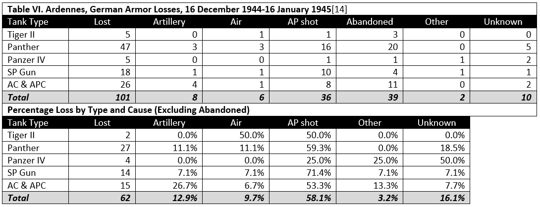
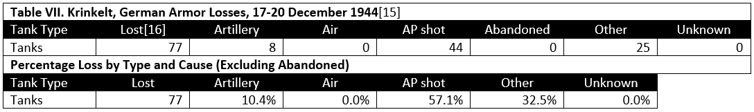
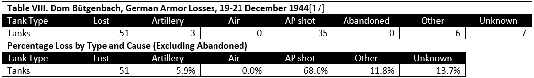
[NOTE: This piece was originally posted on 23 August 2016]

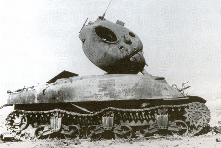
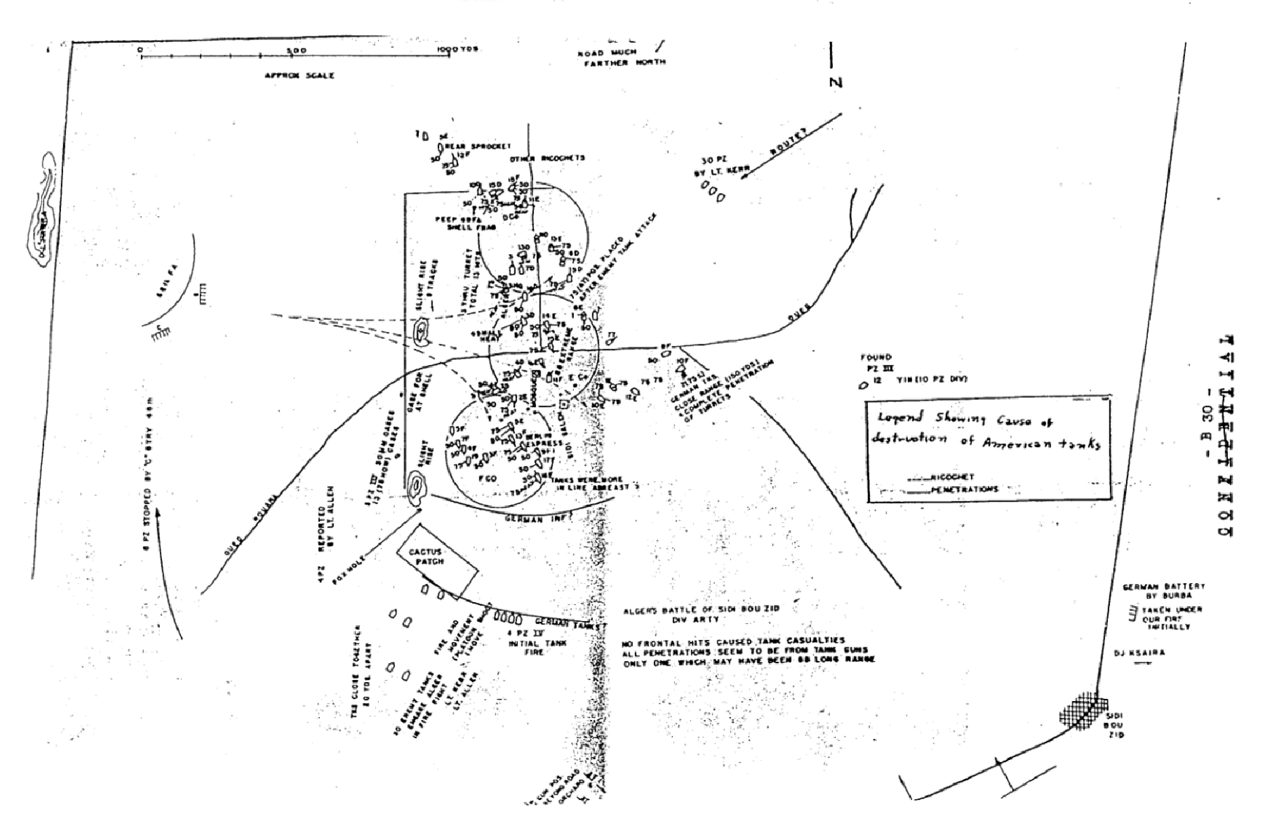
A few years ago, I came across a student battle analysis exercise prepared by the U.S. Army Combat Studies Institute on the Battle of Kasserine Pass in Tunisia in February 1943. At the time, I noted the diagram below (click for larger version), which showed the locations of U.S. tanks knocked out during a counterattack conducted by Combat Command C (CCC) of the U.S. 1st Armored Division against elements of the German 10th and 21st Panzer Divisions near the village of Sidi Bou Zid on 15 February 1943. Without reconnaissance and in the teeth of enemy air superiority, the inexperienced CCC attacked directly into a classic German tank ambush. CCC’s drive on Sidi Bou Zid was halted by a screen of German anti-tank guns, while elements of the two panzer divisions attacked the Americans on both flanks. By the time CCC withdrew several hours later, it had lost 46 of 52 M4 Sherman medium tanks, along with 15 officers and 298 men killed, captured, or missing.

Sidi Bou Zid00
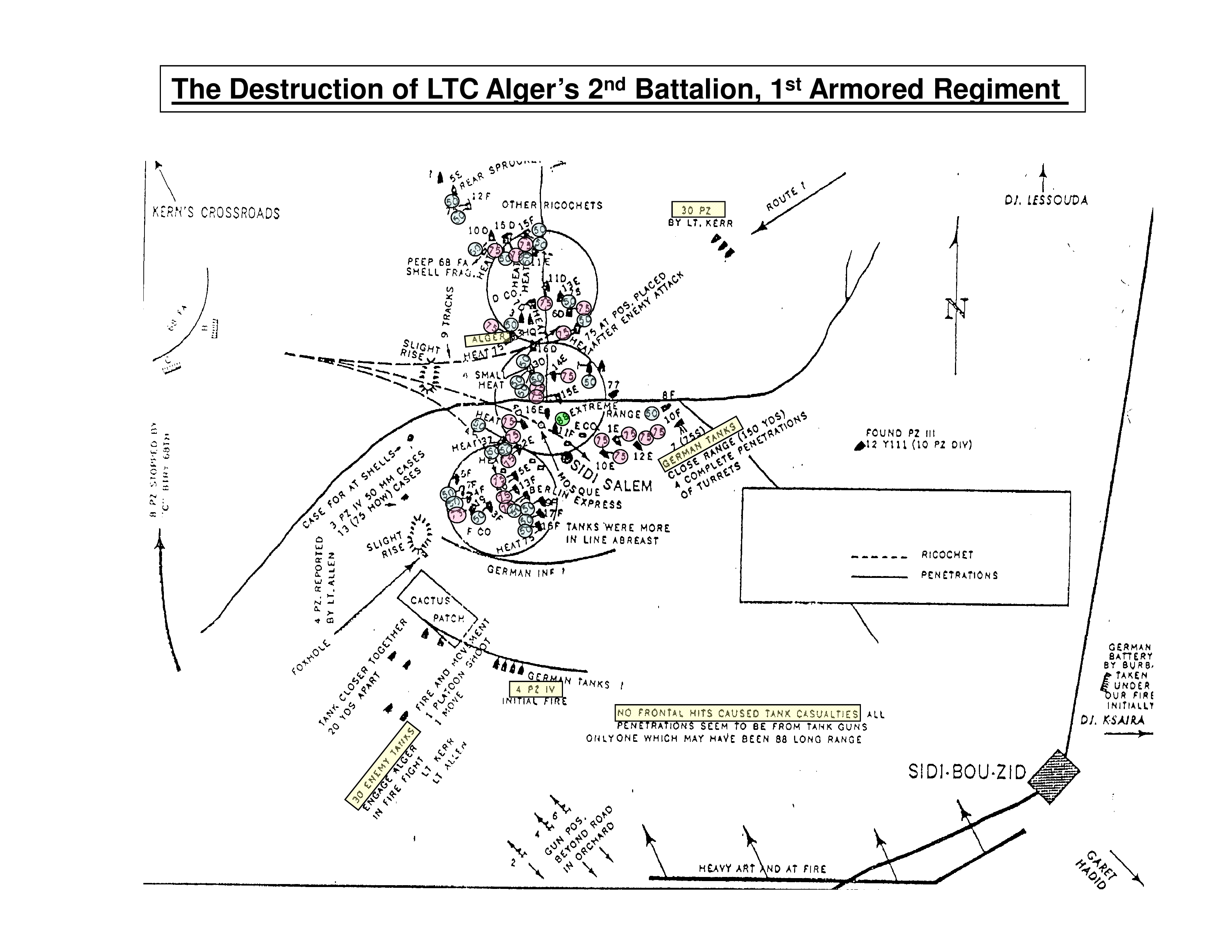
During a recent conversation with my colleague, Chris Lawrence, I recalled the diagram and became curious where it had originated. It identified the location of each destroyed tank, which company it belonged to, and what type of enemy weapon apparently destroyed it; significant battlefield features; and the general locations and movements of the enemy forces. What it revealed was significant. None of CCC’s M4 tanks were disabled or destroyed by a penetration of their frontal armor. Only one was hit by a German 88mm round from either the anti-tank guns or from the handful of available Panzer Mk. VI Tigers. All of the rest were hit with 50mm rounds from Panzer Mk. IIIs, which constituted most of the German force, or by 75mm rounds from Mk. IV’s. The Americans were not defeated by better German tanks. The M4 was superior to the Mk. III and equal to the Mk. IV; the dreaded 88mm anti-tank guns and Tiger tanks played little role in the destruction. The Americans had succumbed to superior German tactics and their own errors.

Counting dead tanks and analyzing their cause of death would have been an undertaking conducted by military operations researchers, at least in the early days of the profession. As Chris pointed out however, the Kasserine battle took place before the inception of operations research in the U.S. Army.

After a bit of digging online, I still have not been able to establish paternity of the diagram, but I think it was created as part of a battlefield survey conducted by the headquarters staff of either the U.S. 1st Armored Division, or one of its subordinate combat commands. The only reference I can find for it is as part of a historical report compiled by Brigadier General Paul Robinett, submitted to support the preparation of Northwest Africa: Seizing the Initiative in the West by George F. Howe, the U.S. Army Center of Military History’s (CMH) official history volume on U.S. Army operations in North Africa, published in 1956. Robinett was the commander of Combat Command B, U.S. 1st Armored Division during the Battle of Kasserine Pass, but did not participate in the engagement at Sidi Bou Zid. His report is excerpted in a set of readings (pp. 103-120) provided as background material for a Kasserine Pass staff ride prepared by CMH. (Curiously, the account of the 15 February engagement at Sidi Bou Zid in Northwest Africa [pp. 419-422] does not reference Robinett’s study.)

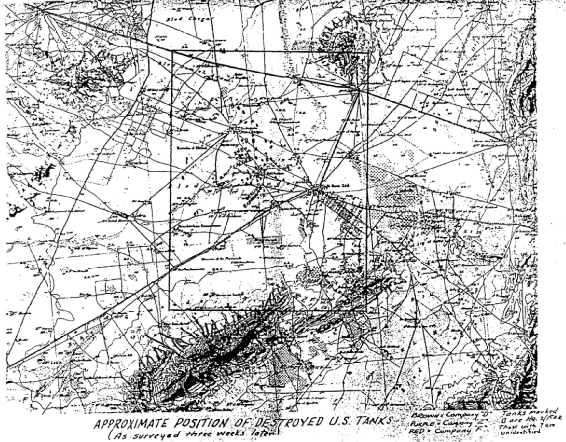
Robinett’s report appeared to include an annotated copy of a topographical map labeled “approximate location of destroyed U.S. tanks (as surveyed three weeks later).” This suggests that the battlefield was surveyed in late March 1943, after U.S. forces had defeated the Germans and regained control of the area.

Sidi Bou Zid02The report also included a version of the schematic diagram later reproduced by CMH. The notes on the map seem to indicate that the survey was the work of staff officers, perhaps at Robinett’s direction, possibly as part of an after-action report.

Sidi Bou Zid03If anyone knows more about the origins of this bit of battlefield archaeology, I would love to know more about it. As far as I know, this assessment was unique, at least in the U.S. Army in World War II.

TDI Friday Read: Tank Combat at Kursk

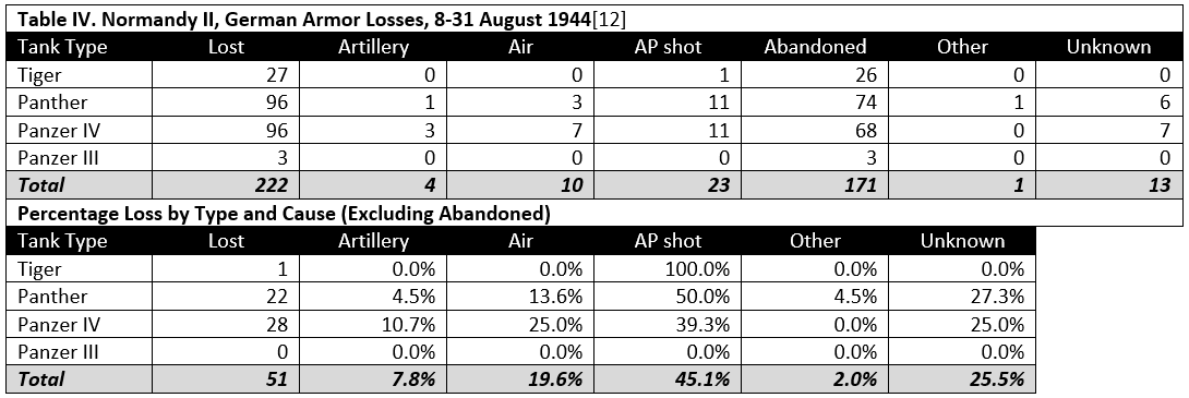
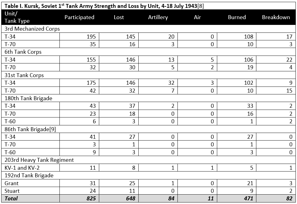
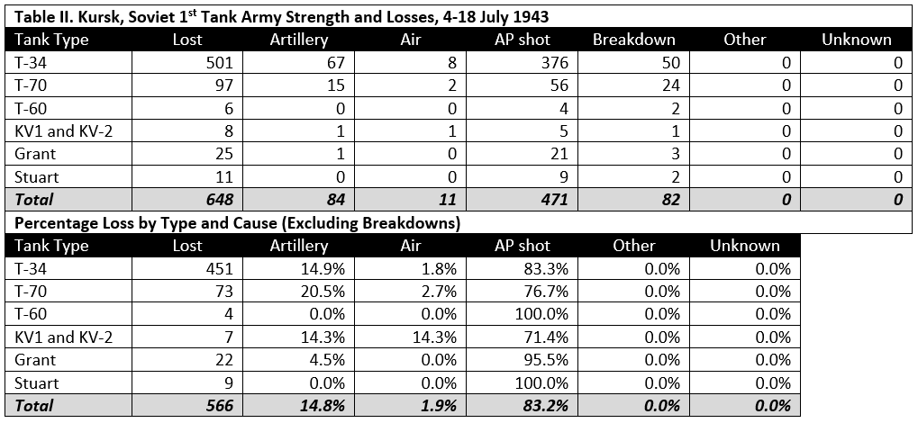
Today’s edition of TDI Friday Read is a roundup of posts by TDI President Christopher Lawrence exploring the details of tank combat between German and Soviet forces at the Battle of Kursk in 1943. The prevailing historical interpretation of Kursk is of the Soviets using their material and manpower superiority to blunt and then overwhelm the German offensive. This view is often buttressed by looking at the  ratio of the numbers of tanks destroyed in combat. Chris takes a deeper look at the data, the differences in the ways “destroyed” tanks were counted and reported, and the differing philosophies between the German and Soviet armies regarding damaged tank recovery and repair. This yields a much more nuanced perspective on the character of tank combat at Kursk that does not necessarily align with the prevailing historical interpretations. Historians often discount detailed observational data on combat as irrelevant or too difficult to collect and interpret. We at TDI believe that with history, the devil is always in the details.

Armor Exchange Ratios at Kursk

Armor Exchange Ratios at Kursk, 5 and 6 July 1943

Soviet Tank Repairs at Kursk (part 1 of 2)

Soviet Tank Repairs at Kursk (part 2 of 2)

German Damaged versus Destroyed Tanks at Kursk

Soviet Damaged versus Destroyed Tanks at Kursk

Comparative Tank Exchange Ratios at Kursk

Japan’s Grand Strategy And The Japanese Air Self Defense Force (JASDF) (III)

[Nippon.com]

Modern air forces require significant capital investments (surpassed only by naval capital investment requirements) and also require significant technological capability. Both of these aspects of modern military power require a strong economic foundation for support. Japan has a long history of investing in its own military industrial capability.

During the Meiji era (1868 to 1912), Japan economic doctrine was summed up in a motto: fukoku kyōhei, meaning “Enrich the Country, Strengthen the Armed Forces.” This phrase actually comes from an ancient Chinese book named Zhan Guo Ce (“Strategies of the Warring States”), from the 5th – 3rd century B.C. period of the same name in Chinese history. This is an excellent example of how for both Japan and China reference their own historical experiences to inform current decision-making.

The post-World War II Japanese body politic had lived through the devastation of war and became focused on economic recovery. The original motto was thus shortened to eliminate kyōhei (“strong army”), leaving only fukoku (“enrich the country”). The resulting single-minded focus paid dividends as the Japanese “economic miracle” enabled it to become the first Asian nation to “catch” the West (see image above). This policy is sometimes referred to as the “Yoshida Doctrine.” Coined in 1977 by Masashi Nishihara and summarized by Professor Sugita of Osaka University, the main elements of the doctrine are:

  1. Japan ensures its national security through an alliance with the United States;
  2. Japan maintains a low capacity for self-defense;
  3. Japan spends resources conserved by the first and second policies on economic activities to develop the country as a trading nation.

In December 2012, Prime Minister Shinzo Abe announced “Abenomics”, a multi-faceted approach to revive Japan’s sluggish economy and to restore Japan’s geopolitical influence as a counterbalance to China’s rise. Abe and his Liberal Democratic Party (LDP) have re-invoked the term fukoku kyōhei, acknowledging that a strong economy and a strong military will be needed in this endeavor.

Japan’s Grand Strategy And The Japanese Air Self Defense Force (JASDF) (II)

Hypothetical occupation zones for post-war Japan had the Allies decided to divide the country. [Pinterest]

In previous posts, I have explored the political and strategic context for the role of the Japan Maritime Self Defense Force (JMSDF). Now I will look at the political reasons why the Japanese Air Self Defense Force (JASDF) is restricted in its operating concepts and capabilities.

After the Pacific War (which for Japan lasted from 1931 to 1945), the devastation of the war and backlash against militarism became conventional wisdom among Japanese. At the Moscow Conference of December 1945, the Allies agreed that since Japan had fallen to the United States, that country would be allowed to conduct the post-war occupation. (Hungary had fallen to the Red Army and thus was occupied by the Soviet Union alone.) This decision saved Japan from a division like Germany or Korea, although the Soviets still had plans for a Japanese communist state (see below). The map above is a hypothetical division of Japan, developed by a wargamer.

The greater Japanese empire, however was divided among the Allies, with many natural choices, such as the former British colonial possessions being returned (e.g. Singapore, Hong Kong, etc.), former French colonial possessions being returned (Indochina), South Sakhalin and the Kuril Islands going to the Soviets, and Taiwan and the Pescadores returning to China (although which China became a key question in 1949). Notably, Korea was divided into North and South, with the Soviets in control of the former, and the other Allies (primarily the US and UK) managing the later.

In Japan, the Supreme Commander for the Allied Powers (SCAP), General Douglas MacArthur governed and imposed a new post-war constitution, which came into force in May 1947, and is technically an amendment to the original Meiji-era constitution of 1889. Article 9 of which reads as below:

(1) Aspiring sincerely to an international peace based on justice and order, the Japanese people forever renounce war as a sovereign right of the nation and the threat or use of force as means of settling international disputes.

(2) In order to accomplish the aim of the preceding paragraph, land, sea, and air forces, as well as other war potential, will never be maintained. The right of belligerency of the state will not be recognized.

As early as 1946, however, planners in the the Joint Staff, under the U.S. Joint Chiefs of Staff (JCS), began to consider the re-armament of Japan, anticipating a Soviet attack against Japan. The actual Soviet war plan to attack Hokkaido on August 24th 1945 was published by the Wilson center in 2015, and some say that strategic nuclear deterrence was what saved Japan from the same fate as divided Germany.

In March 1948, when Washington considered starting peace treaty negotiations with Japan, Under Secretary of the Army William Draper stated that the War Department was generally in favor of Japanese rearmament. In response to an inquiry by the secretary of defense, the JCS stated: ‘Solely from the military viewpoint, the establishment of Japanese armed forces is desirable’ to offset ‘our own limited manpower.’

The American vision of an unarmed and pacifist Japan, as rapidly enshrined in the constitution, was nearly dead on arrival, as international events unfolded rapidly in the late 1940’s and early 1950’s:

  • 1947, March – President Harry Truman addressed Congress and the U.S. public, announcing the policy of containment, and establishing the Truman Doctrine.
  • June 1948 – the Soviet Union blockaded Berlin, resulting in the famous airlift.
  • October 1949 – Chiang Kai-shek and the Republic of China were defeated by Mao Zedong and the Chinese Red Army, founding the People’s Republic of China (PRC).
  • June 1950 – North Korea, a Soviet satellite state since 1945, invaded South Korea, fracturing the post-war territorial division.

Thus, by 1950 when John Foster Dulles was appointed to begin negotiating a peace treaty with Japan to conclude the American occupation, he and most other American policy makers had come to see Japan as very important to the defense of American interests and democracy in the Far East.

  • September 1951 – The Treaty of San Francisco was signed, establishing peace between Japan and many Allied nations, but notably not the Soviet Union, China as Republic of China (Taiwan), or People’s Republic of China (mainland), or North nor South Korea.
  • September 1951 – The U.S.-Japan Security Treaty was signed on the same date, but entered into force in April 1952. This ended the military occupation, restored sovereignty to the Japanese government, but also clarified the ongoing US military presence in Japan, originally the Far East Command (FEC) from 1947 until 1957 when the United States Forces Japan (USFJ).
  • March 1954 – The original Treaty of Mutual Cooperation and Security between the United States and Japan, “contained provisions that permitted the United States to act for the sake of maintaining peace in East Asia and even exert its power on Japanese domestic quarrels.” (Wikipedia)
  • October 1956 – The Soviet Union and Japan signed the Joint Declaration, a bi-lateral agreement short of a peace treaty. This normalized relations between the countries since the Soviet Union did not sign the 1951 Treaty of San Francisco. This agreement breaks news today, as Japan and Russia are currently moving towards a peace treaty.
  • 1958 – The U.S. Air Force (USAF) handed over airspace responsibility to JASDF. Threats to Japanese airspace were dealt with in the same way that they were in the U.S. prior to the Semi-Automatic Ground Environment (SAGE) system, much like they were by the British in 1940 (see Dowding System), by manual means. It would be more than a decade until Japan had its own version of SAGE, known as Base Air Defense Ground Environment (BADGE) in English, and 自動警戒管制組織 (jidou keikai kansei soshiki) ”Automatic Warning and Control Organization” in Japanese. [More on this in a future post.]
  • January 1960 – Two key documents were updated, the Treaty of Mutual Cooperation and Security, and the U.S.-Japan Status of Forces Agreement. To alleviate the unequal status, removed the provision to intervene in Japanese domestic quarrels, included articles to delineate mutual defense obligations, and U.S. obligations to pre-inform Japan in times of the U.S. military mobilization. The ratification of this treaty was greeted with widespread protests by the Japanese public, who opposed nuclear weapons in Japan, and were concerned about being on the front line in a possible nuclear exchange between the US and the Soviet Union.

Historians and the Early Era of U.S. Army Operations Research

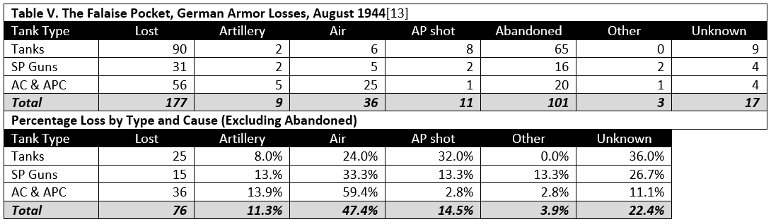
While perusing Charles Shrader’s fascinating history of the U.S. Army’s experience with operations research (OR), I came across several references to the part played by historians and historical analysis in early era of that effort.

The ground forces were the last branch of the Army to incorporate OR into their efforts during World War II, lagging behind the Army Air Forces, the technical services, and the Navy. Where the Army was a step ahead, however, was in creating a robust wartime historical field history documentation program. (After the war, this enabled the publication of the U.S. Army in World War II series, known as the “Green Books,” which set a new standard for government sponsored military histories.)

As Shrader related, the first OR personnel the Army deployed forward in 1944-45 often crossed paths with War Department General Staff Historical Branch field historian detachments. They both engaged in similar activities: collecting data on real-world combat operations, which was then analyzed and used for studies and reports written for the use of the commands to which they were assigned. The only significant difference was in their respective methodologies, with the historians using historical methods and the OR analysts using mathematical and scientific tools.

History and OR after World War II

The usefulness of historical approaches to collecting operational data did not go unnoticed by the OR practitioners, according to Shrader. When the Army established the Operations Research Office (ORO) in 1948, it hired a contingent of historians specifically for the purpose of facilitating research and analysis using WWII Army records, “the most likely source for data on operational matters.”

When the Korean War broke out in 1950, ORO sent eight multi-disciplinary teams, including the historians, to collect operational data and provide analytical support for U.S. By 1953, half of ORO’s personnel had spent time in combat zones. Throughout the 1950s, about 40-43% of ORO’s staff was comprised of specialists in the social sciences, history, business, literature, and law. Shrader quoted one leading ORO analyst as noting that, “there is reason to believe that the lawyer, social scientist or historian is better equipped professionally to evaluate evidence which is derived from the mind and experience of the human species.”

Among the notable historians who worked at or with ORO was Dr. Hugh M. Cole, an Army officer who had served as a staff historian for General George Patton during World War II. Cole rose to become a senior manager at ORO and later served as vice-president and president of ORO’s successor, the Research Analysis Corporation (RAC). Cole brought in WWII colleague Forrest C. Pogue (best known as the biographer of General George C. Marshall) and Charles B. MacDonald. ORO also employed another WWII field historian, the controversial S. L. A. Marshall, as a consultant during the Korean War. Dorothy Kneeland Clark did pioneering historical analysis on combat phenomena while at ORO.

The Demise of ORO…and Historical Combat Analysis?

By the late 1950s, considerable institutional friction had developed between ORO, the Johns Hopkins University (JHU)—ORO’s institutional owner—and the Army. According to Shrader,

Continued distrust of operations analysts by Army personnel, questions about the timeliness and focus of ORO studies, the ever-expanding scope of ORO interests, and, above all, [ORO director] Ellis Johnson’s irascible personality caused tensions that led in August 1961 to the cancellation of the Army’s contract with JHU and the replacement of ORO with a new, independent research organization, the Research Analysis Corporation [RAC].

RAC inherited ORO’s research agenda and most of its personnel, but changing events and circumstances led Army OR to shift its priorities away from field collection and empirical research on operational combat data in favor of the use of modeling and wargaming in its analyses. As Chris Lawrence described in his history of federally-funded Defense Department “think tanks,” the rise and fall of scientific management in DOD, the Vietnam War, social and congressional criticism, and an unhappiness by the military services with the analysis led to retrenchment in military OR by the end of the 60s. The Army sold RAC and created its own in-house Concepts Analysis Agency (CAA; now known as the Center for Army Analysis).

By the early 1970s, analysts, such as RAND’s Martin Shubik and Gary Brewer, and John Stockfisch, began to note that the relationships and processes being modeled in the Army’s combat simulations were not based on real-world data and that empirical research on combat phenomena by the Army OR community had languished. In 1991, Paul Davis and Donald Blumenthal gave this problem a name: the “Base of Sand.”

Quantifying the Holocaust

Odilo Globocnik, SS and Police Leader in the Lublin district of the General Government territory in German-occupied Poland, was placed in charge of Operation Reinhardt by SS Reichsführer Heinrich Himmler. [Wikipedia]

The devastation and horror of the Holocaust makes it difficult to truly wrap one’s head around its immense scale. Six million murdered Jews is a number so large that it is hard to comprehend, much less understand in detail. While there are many accounts of individual experiences, the wholesale destruction of the Nazi German documentation of their genocide has made it difficult to gauge the dynamics of their activities.

However, in a new study, Lewi Stone, Professor of Biomathematics at RMIT University in Australia, has used an obscure railroad dataset to reconstruct the size and scale of a specific action by the Germans in eastern Poland and western Ukraine in 1942. “Quantifying the Holocaust: Hyperintense kill rates during the Nazi genocide,” (Not paywalled. Yet.) published on 2 January in the journal Science Advances, uses train schedule data published in 1987 by historian Yitzhak Arad to track the geographical and temporal dimensions of some 1.7 Jews transported to the Treblinka, Belzec and Sobibor death camps in the late summer and early autumn of 1942.

This action, known as Operation Reinhardt, originated during the Wansee Conference in January 1942 as the plan to carry out Hitler’s Final Solution to exterminate Europe’s Jews. In July, Hitler “ordered all action speeded up” which led to a frenzy of roundups by SS (Schutzstaffel) groups from over 400 Jewish communities in Poland and Ukraine, and transport via 500 trains to the three camps along the Polish-Soviet border. In just 100 days, 1.7 million people had been relocated and almost 1.5 million of them were murdered (“special treatment” (Sonderbehandlung)), most upon arrival at the camps. This phase of Reinhardt came to an end in November 1942 because the Nazis had run out of people to kill.

This three-month period was by far the most intensely murderous phase of the Holocaust, carried out simultaneously with the German summer military offensive that culminated in disastrous battlefield defeat at the hands of the Soviets at Stalingrad at year’s end. 500,000 Jews were killed per month, or an average of 15,000 per day. Even parsed from the overall totals, these numbers remain hard to grasp.

Stone’s research is innovative and sobering. His article can currently be downloaded in PDF format. His piece in The Conversation includes interactive online charts. He also produced a video the presents his findings chronologically and spatially:

Artillery Effectiveness vs. Armor (Part 5-Summary)

U.S. Army 155mm field howitzer in Normandy. [padresteve.com]

[This series of posts is adapted from the article “Artillery Effectiveness vs. Armor,” by Richard C. Anderson, Jr., originally published in the June 1997 edition of the International TNDM Newsletter.]

Posts in the series
Artillery Effectiveness vs. Armor (Part 1)
Artillery Effectiveness vs. Armor (Part 2-Kursk)
Artillery Effectiveness vs. Armor (Part 3-Normandy)
Artillery Effectiveness vs. Armor (Part 4-Ardennes)
Artillery Effectiveness vs. Armor (Part 5-Summary)

Table IX shows the distribution of cause of loss by type or armor vehicle. From the distribution it might be inferred that better protected armored vehicles may be less vulnerable to artillery attack. Nevertheless, the heavily armored vehicles still suffered a minimum loss of 5.6 percent due to artillery. Unfortunately the sample size for heavy tanks was very small, 18 of 980 cases or only 1.8 percent of the total.

The data are limited at this time to the seven cases.[6] Further research is necessary to expand the data sample so as to permit proper statistical analysis of the effectiveness of artillery versus tanks.

NOTES

[18] Heavy armor includes the KV-1, KV-2, Tiger, and Tiger II.

[19] Medium armor includes the T-34, Grant, Panther, and Panzer IV.

[20] Light armor includes the T-60, T-70. Stuart, armored cars, and armored personnel carriers.

Artillery Effectiveness vs. Armor (Part 4-Ardennes)

Knocked-out Panthers in Krinkelt, Belgium, Battle of the Bulge, 17 December 1944. [worldwarphotos.info]

[This series of posts is adapted from the article “Artillery Effectiveness vs. Armor,” by Richard C. Anderson, Jr., originally published in the June 1997 edition of the International TNDM Newsletter.]

Posts in the series
Artillery Effectiveness vs. Armor (Part 1)
Artillery Effectiveness vs. Armor (Part 2-Kursk)
Artillery Effectiveness vs. Armor (Part 3-Normandy)
Artillery Effectiveness vs. Armor (Part 4-Ardennes)
Artillery Effectiveness vs. Armor (Part 5-Summary)

NOTES

[14] From ORS Joint Report No. 1. A total of an estimated 300 German armor vehicles were found following the battle.

[15] Data from 38th Infantry After Action Report (including “Sketch showing enemy vehicles destroyed by 38th Inf Regt. and attached units 17-20 Dec. 1944″), from 12th SS PzD strength report dated 8 December 1944, and from strengths indicated on the OKW briefing maps for 17 December (1st [circa 0600 hours], 2d [circa 1200 hours], and 3d [circa 1800 hours] situation), 18 December (1st and 2d situation), 19 December (2d situation), 20 December (3d situation), and 21 December (2d and 3d situation).

[16] Losses include confirmed and probable losses.

[17] Data from Combat Interview “26th Infantry Regiment at Dom Bütgenbach” and from 12th SS PzD, ibid.

Artillery Effectiveness vs. Armor (Part 3-Normandy)

The U.S. Army 333rd Field Artillery Battalion (Colored) in Normandy, July 1944 (US Army Photo/Tom Gregg)

[This series of posts is adapted from the article “Artillery Effectiveness vs. Armor,” by Richard C. Anderson, Jr., originally published in the June 1997 edition of the International TNDM Newsletter.]

Posts in the series
Artillery Effectiveness vs. Armor (Part 1)
Artillery Effectiveness vs. Armor (Part 2-Kursk)
Artillery Effectiveness vs. Armor (Part 3-Normandy)
Artillery Effectiveness vs. Armor (Part 4-Ardennes)
Artillery Effectiveness vs. Armor (Part 5-Summary)

NOTES

[10] From ORS Report No. 17.

[11] Five of the 13 counted as unknown were penetrated by both armor piercing shot and by infantry hollow charge weapons. There was no evidence to indicate which was the original cause of the loss.

[12] From ORS Report No. 17

[13] From ORS Report No. 15. The “Pocket” was the area west of the line Falaise-Argentan and east of the line Vassy-Gets-Domfront in Normandy that was the site in August 1944 of the beginning of the German retreat from France. The German forces were being enveloped from the north and south by Allied ground forces and were under constant, heavy air attack.

Artillery Effectiveness vs. Armor (Part 2-Kursk)

15 cm schwere Feldhaubitze 18 (15 cm s.FH 18 L/29,5)

German Army 150mm heavy field howitzer 18 L/29.5 battery. [Panzer DB/Pinterest]

[This series of posts is adapted from the article “Artillery Effectiveness vs. Armor,” by Richard C. Anderson, Jr., originally published in the June 1997 edition of the International TNDM Newsletter.]

Posts in the series
Artillery Effectiveness vs. Armor (Part 1)
Artillery Effectiveness vs. Armor (Part 2-Kursk)
Artillery Effectiveness vs. Armor (Part 3-Normandy)
Artillery Effectiveness vs. Armor (Part 4-Ardennes)
Artillery Effectiveness vs. Armor (Part 5-Summary)

Curiously, at Kursk, in the case where the highest percent loss was recorded, the German forces opposing the Soviet 1st Tank Army—mainly the XLVIII Panzer Corps of the Fourth Panzer Army—were supported by proportionately fewer artillery pieces (approximately 56 guns and rocket launchers per division) than the US 1st Infantry Division at Dom Bütgenbach (the equivalent of approximately 106 guns per division)[4]. Nor does it appear that the German rate of fire at Kursk was significantly higher than that of the American artillery at Dom Bütgenbach. On 20 July at Kursk, the 150mm howitzers of the 11th Panzer Division achieved a peak rate of fire of 87.21 rounds per gum. On 21 December at Dom Bütgenbach, the 155mm howitzers of the 955th Field Artillery Battalion achieved a peak rate of fire of 171.17 rounds per gun.[5]

NOTES

[4] The US artillery at Dom Bütgenbach peaked on 21 December 1944 when a total of 210 divisional and corps pieces fired over 10,000 rounds in support of the 1st Division’s 26th Infantry.

[5] Data collected on German rates of fire are fragmentary, but appear to be similar to that of the American Army in World War ll. An article on artillery rates of fire that explores the data in more detail will be forthcoming in a future issue of this newsletter. [NOTE: This article was not completed or published.]

Notes to Table I.

[8] The data were found in reports of the 1st Tank Army (Fond 299, Opis‘ 3070, Delo 226). Obvious math errors in the original document have been corrected (the total lost column did not always agree with the totals by cause). The total participated column evidently reflected the starting strength of the unit, plus replacement vehicles. “Burned'” in Soviet wartime documents usually indicated a total loss, however it appears that in this case “burned” denoted vehicles totally lost due to direct fire antitank weapons. “Breakdown” apparently included both mechanical breakdown and repairable combat damage.

[9] Note that the brigade report (Fond 3304, Opis‘ 1, Delo 24) contradicts the army report. The brigade reported that a total of 28 T-34s were lost (9 to aircraft and 19 to “artillery”) and one T-60 was destroyed by a mine. However, this report was made on 11 July, during the battle, and may not have been as precise as the later report recorded by 1st Tank Army. Furthermore, it is not as clear in the brigade report that “artillery” referred only to indirect fire HE and not simply lo both direct and indirect fire guns.