 [The article below is reprinted from Winter 2010 edition of The International TNDM Newsletter.]
A Summation of QJM/TNDM Validation Efforts
By Christopher A. Lawrence
There have been six or seven different validation tests conducted of the QJM (Quantified Judgment Model) and the TNDM (Tactical Numerical Deterministic Model). As the changes to these two models are evolutionary in nature but do not fundamentally change the nature of the models, the whole series of validation tests across both models is worth noting. To date, this is the only model we are aware of that has been through multiple validations. We are not aware of any DOD [Department of Defense] combat model that has undergone more than one validation effort. Most of the DOD combat models in use have not undergone any validation.
The Two Original Validations of the QJM
After its initial development using a 60-engagement WWII database, the QJM was tested in 1973 by application of its relationships and factors to a validation database of 21 World War II engagements in Northwest Europe in 1944 and 1945. The original model proved to be 95% accurate in explaining the outcomes of these additional engagements. Overall accuracy in predicting the results of the 81 engagements in the developmental and validation databases was 93%.[1]
During the same period the QJM was converted from a static model that only predicted success or failure to one capable of also predicting attrition and movement. This was accomplished by adding variables and modifying factor values. The original QJM structure was not changed in this process. The addition of movement and attrition as outputs allowed the model to be used dynamically in successive “snapshot” iterations of the same engagement.
From 1973 to 1979 the QJM’s formulae, procedures, and variable factor values were tested against the results of all of the 52 significant engagements of the 1967 and 1973 Arab-Israeli Wars (19 from the former, 33 from the latter). The QJM was able to replicate all of those engagements with an accuracy of more than 90%?[2]
In 1979 the improved QJM was revalidated by application to 66 engagements. These included 35 from the original 81 engagements (the “development database”), and 31 new engagements. The new engagements included five from World War II and 26 from the 1973 Middle East War. This new validation test considered four outputs: success/failure, movement rates, personnel casualties, and tank losses. The QJM predicted success/failure correctly for about 85% of the engagements. It predicted movement rates with an error of 15% and personnel attrition with an error of 40% or less. While the error rate for tank losses was about 80%, it was discovered that the model consistently underestimated tank losses because input data included all kinds of armored vehicles, but output data losses included only numbers of tanks.[3]
This completed the original validations efforts of the QJM. The data used for the validations, and parts of the results of the validation, were published, but no formal validation report was issued. The validation was conducted in-house by Colonel Dupuy’s organization, HERO [Historical Evaluation Research Organization]. The data used were mostly from division-level engagements, although they included some corps- and brigade-level actions. We count these as two separate validation efforts.
The Development of the TNDM and Desert Storm
In 1990 Col. Dupuy, with the collaborative assistance of Dr. James G. Taylor (author of Lanchester Models of Warfare [vol. 1] [vol. 2], published by the Operations Research Society of America, Arlington, Virginia, in 1983) introduced a significant modification: the representation of the passage of time in the model. Instead of resorting to successive “snapshots,” the introduction of Taylor’s differential equation technique permitted the representation of time as a continuous flow. While this new approach required substantial changes to the software, the relationship of the model to historical experience was unchanged.[4] This revision of the model also included the substitution of formulae for some of its tables so that there was a continuous flow of values across the individual points in the tables. It also included some adjustment to the values and tables in the QJM. Finally, it incorporated a revised OLI [Operational Lethality Index] calculation methodology for modem armor (mobile fighting machines) to take into account all the factors that influence modern tank warfare.[5] The model was reprogrammed in Turbo PASCAL (the original had been written in BASIC). The new model was called the TNDM (Tactical Numerical Deterministic Model).
Building on its foundation of historical validation and proven attrition methodology, in December 1990, HERO used the TNDM to predict the outcome of, and losses from, the impending Operation DESERT STORM.[6] It was the most accurate (lowest) public estimate of U.S. war casualties provided before the war. It differed from most other public estimates by an order of magnitude.
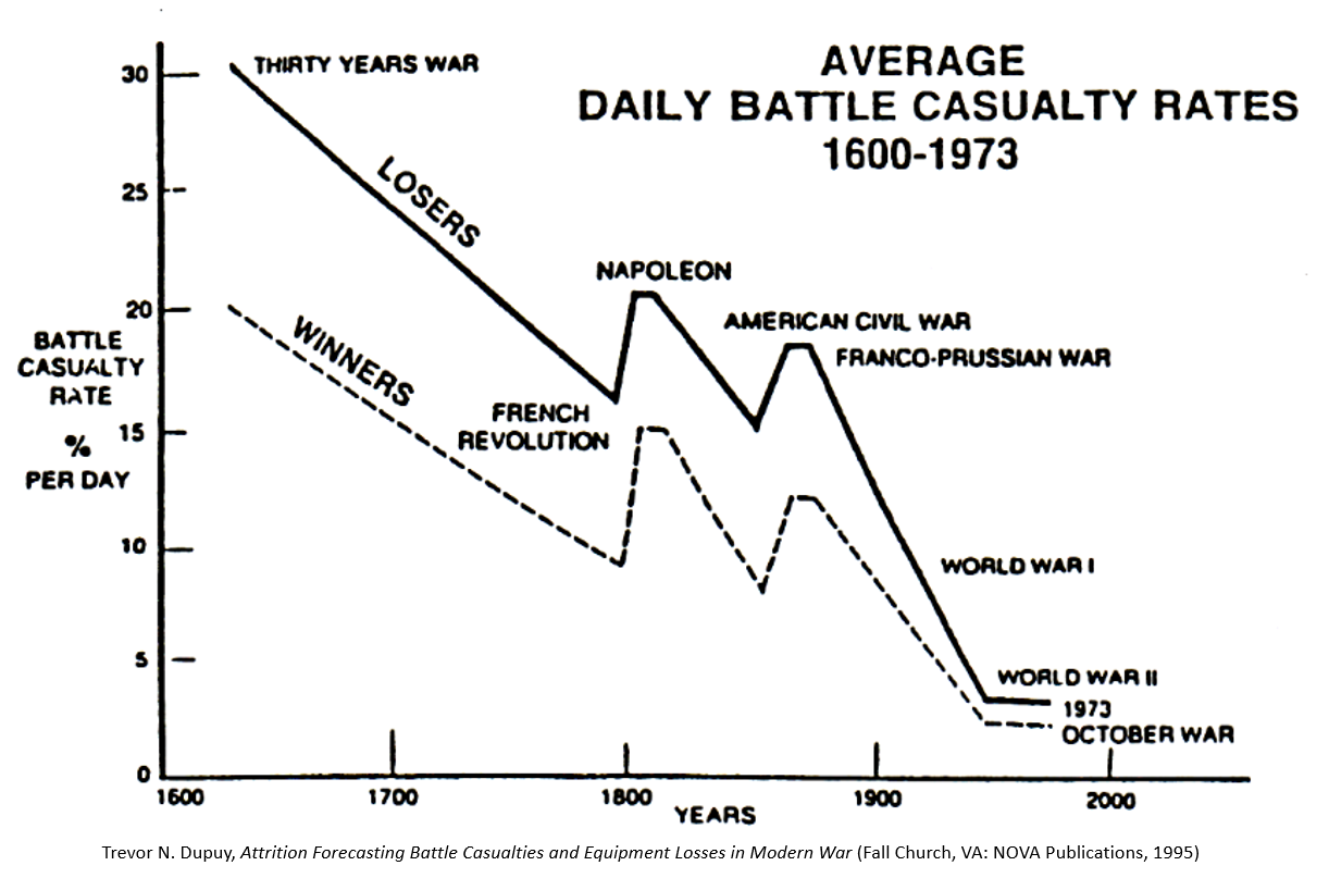
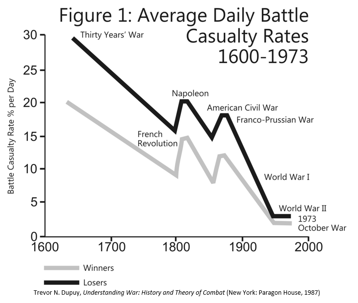
Also, in 1990, Trevor Dupuy published an abbreviated form of the TNDM in the book Attrition: Forecasting Battle Casualties and Equipment Losses in Modern War. A brief validation exercise using 12 battles from 1805 to 1973 was published in this book.[7] This version was used for creation of M-COAT[8] and was also separately tested by a student (Lieutenant Gozel) at the Naval Postgraduate School in 2000.[9] This version did not have the firepower scoring system, and as such neither M-COAT, Lieutenant Gozel’s test, nor Colonel Dupuy’s 12-battle validation included the OLI methodology that is in the primary version of the TNDM.
For counting purposes, I consider the Gulf War the third validation of the model. In the end, for any model, the proof is in the pudding. Can the model be used as a predictive tool or not? If not, then there is probably a fundamental flaw or two in the model. Still the validation of the TNDM was somewhat second-hand, in the sense that the closely-related previous model, the QJM, was validated in the 1970s to 200 World War II and 1967 and 1973 Arab-Israeli War battles, but the TNDM had not been. Clearly, something further needed to be done.
The Battalion-Level Validation of the TNDM
Under the guidance of Christopher A. Lawrence, The Dupuy Institute undertook a battalion-level validation of the TNDM in late 1996. This effort tested the model against 76 engagements from World War I, World War II, and the post-1945 world including Vietnam, the Arab-Israeli Wars, the Falklands War, Angola, Nicaragua, etc. This effort was thoroughly documented in The International TNDM Newsletter.[10] This effort was probably one of the more independent and better-documented validations of a casualty estimation methodology that has ever been conducted to date, in that:
- The data was independently assembled (assembled for other purposes before the validation) by a number of different historians.
- There were no calibration runs or adjustments made to the model before the test.
- The data included a wide range of material from different conflicts and times (from 1918 to 1983).
- The validation runs were conducted independently (Susan Rich conducted the validation runs, while Christopher A. Lawrence evaluated them).
- The results of the validation were fully published.
- The people conducting the validation were independent, in the sense that:
a) there was no contract, management, or agency requesting the validation;
b) none of the validators had previously been involved in designing the model, and had only very limited experience in using it; and
c) the original model designer was not able to oversee or influence the validation.[11]
The validation was not truly independent, as the model tested was a commercial product of The Dupuy Institute, and the person conducting the test was an employee of the Institute. On the other hand, this was an independent effort in the sense that the effort was employee-initiated and not requested or reviewed by the management of the Institute. Furthermore, the results were published.
The TNDM was also given a limited validation test back to its original WWII data around 1997 by Niklas Zetterling of the Swedish War College, who retested the model to about 15 or so Italian campaign engagements. This effort included a complete review of the historical data used for the validation back to their primarily sources, and details were published in The International TNDM Newsletter.[12]
There has been one other effort to correlate outputs from QJM/TNDM-inspired formulae to historical data using the Ardennes and Kursk campaign-level (i.e., division-level) databases.[13] This effort did not use the complete model, but only selective pieces of it, and achieved various degrees of “goodness of fit.” While the model is hypothetically designed for use from squad level to army group level, to date no validation has been attempted below battalion level, or above division level. At this time, the TNDM also needs to be revalidated back to its original WWII and Arab-Israeli War data, as it has evolved since the original validation effort.
The Corps- and Division-level Validations of the TNDM
Having now having done one extensive battalion-level validation of the model and published the results in our newsletters, Volume 1, issues 5 and 6, we were then presented an opportunity in 2006 to conduct two more validations of the model. These are discussed in depth in two articles of this issue of the newsletter.
These validations were again conducted using historical data, 24 days of corps-level combat and 25 cases of division-level combat drawn from the Battle of Kursk during 4-15 July 1943. It was conducted using an independently-researched data collection (although the research was conducted by The Dupuy Institute), using a different person to conduct the model runs (although that person was an employee of the Institute) and using another person to compile the results (also an employee of the Institute). To summarize the results of this validation (the historical figure is listed first followed by the predicted result):
 There was one other effort that was done as part of work we did for the Army Medical Department (AMEDD). This is fully explained in our report Casualty Estimation Methodologies Study: The Interim Report dated 25 July 2005. In this case, we tested six different casualty estimation methodologies to 22 cases. These consisted of 12 division-level cases from the Italian Campaign (4 where the attack failed, 4 where the attacker advanced, and 4 Where the defender was penetrated) and 10 cases from the Battle of Kursk (2 cases Where the attack failed, 4 where the attacker advanced and 4 where the defender was penetrated). These 22 cases were randomly selected from our earlier 628 case version of the DLEDB (Division-level Engagement Database; it now has 752 cases). Again, the TNDM performed as well as or better than any of the other casualty estimation methodologies tested. As this validation effort was using the Italian engagements previously used for validation (although some had been revised due to additional research) and three of the Kursk engagements that were later used for our division-level validation, then it is debatable whether one would want to call this a seventh validation effort. Still, it was done as above with one person assembling the historical data and another person conducting the model runs. This effort was conducted a year before the corps and division-level validation conducted above and influenced it to the extent that we chose a higher CEV (Combat Effectiveness Value) for the later validation. A CEV of 2.5 was used for the Soviets for this test, vice the CEV of 3.0 that was used for the later tests.
Summation
The QJM has been validated at least twice. The TNDM has been tested or validated at least four times, once to an upcoming, imminent war, once to battalion-level data from 1918 to 1989, once to division-level data from 1943 and once to corps-level data from 1943. These last four validation efforts have been published and described in depth. The model continues, regardless of which validation is examined, to accurately predict outcomes and make reasonable predictions of advance rates, loss rates and armor loss rates. This is regardless of level of combat (battalion, division or corps), historic period (WWI, WWII or modem), the situation of the combats, or the nationalities involved (American, German, Soviet, Israeli, various Arab armies, etc.). As the QJM, the model was effectively validated to around 200 World War II and 1967 and 1973 Arab-Israeli War battles. As the TNDM, the model was validated to 125 corps-, division-, and battalion-level engagements from 1918 to 1989 and used as a predictive model for the 1991 Gulf War. This is the most extensive and systematic validation effort yet done for any combat model. The model has been tested and re-tested. It has been tested across multiple levels of combat and in a wide range of environments. It has been tested where human factors are lopsided, and where human factors are roughly equal. It has been independently spot-checked several times by others outside of the Institute. It is hard to say what more can be done to establish its validity and accuracy.
NOTES
[1] It is unclear what these percentages, quoted from Dupuy in the TNDM General Theoretical Description, specify. We suspect it is a measurement of the model’s ability to predict winner and loser. No validation report based on this effort was ever published. Also, the validation figures seem to reflect the results after any corrections made to the model based upon these tests. It does appear that the division-level validation was “incremental.” We do not know if the earlier validation tests were tested back to the earlier data, but we have reason to suspect not.
[2] The original QJM validation data was first published in the Combat Data Subscription Service Supplement, vol. 1, no. 3 (Dunn Loring VA: HERO, Summer 1975). (HERO Report #50) That effort used data from 1943 through 1973.
[3] HERO published its QJM validation database in The QJM Data Base (3 volumes) Fairfax VA: HERO, 1985 (HERO Report #100).
[4] The Dupuy Institute, The Tactical Numerical Deterministic Model (TNDM): A General and Theoretical Description, McLean VA: The Dupuy Institute, October 1994.
[5] This had the unfortunate effect of undervaluing WWII-era armor by about 75% relative to other WWII weapons when modeling WWII engagements. This left The Dupuy Institute with the compromise methodology of using the old OLI method for calculating armor (Mobile Fighting Machines) when doing WWII engagements and using the new OLI method for calculating armor when doing modem engagements
[6] Testimony of Col. T. N. Dupuy, USA, Ret, Before the House Armed Services Committee, 13 Dec 1990. The Dupuy Institute File I-30, “Iraqi Invasion of Kuwait.”
[7] Trevor N. Dupuy, Attrition: Forecasting Battle Casualties and Equipment Losses in Modern War (HERO Books, Fairfax, VA, 1990), 123-4.
[8] M-COAT is the Medical Course of Action Tool created by Major Bruce Shahbaz. It is a spreadsheet model based upon the elements of the TNDM provided in Dupuy’s Attrition (op. cit.) It used a scoring system derived from elsewhere in the U.S. Army. As such, it is a simplified form of the TNDM with a different weapon scoring system.
[9] See Gözel, Ramazan. “Fitting Firepower Score Models to the Battle of Kursk Data,” NPGS Thesis. Monterey CA: Naval Postgraduate School.
[10] Lawrence, Christopher A. “Validation of the TNDM at Battalion Level.” The International TNDM Newsletter, vol. 1, no. 2 (October 1996); Bongard, Dave “The 76 Battalion-Level Engagements.” The International TNDM Newsletter, vol. 1, no. 4 (February 1997); Lawrence, Christopher A. “The First Test of the TNDM Battalion-Level Validations: Predicting the Winner” and “The Second Test of the TNDM Battalion-Level Validations: Predicting Casualties,” The International TNDM Newsletter, vol. 1 no. 5 (April 1997); and Lawrence, Christopher A. “Use of Armor in the 76 Battalion-Level Engagements,” and “The Second Test of the Battalion-Level Validation: Predicting Casualties Final Scorecard.” The International TNDM Newsletter, vol. 1, no. 6 (June 1997).
[11] Trevor N. Dupuy passed away in July 1995, and the validation was conducted in 1996 and 1997.
[12] Zetterling, Niklas. “CEV Calculations in Italy, 1943,” The International TNDM Newsletter, vol. 1, no. 6. McLean VA: The Dupuy Institute, June 1997. See also Research Plan, The Dupuy Institute Report E-3, McLean VA: The Dupuy Institute, 7 Oct 1998.
[13] See Gözel, “Fitting Firepower Score Models to the Battle of Kursk Data.”
 “If we maintain our faith in God, love of freedom, and superior global airpower, the future [of the US] looks good.” — U.S. Air Force General Curtis E. LeMay (Commander, U.S. Strategic Command, 1948-1957)
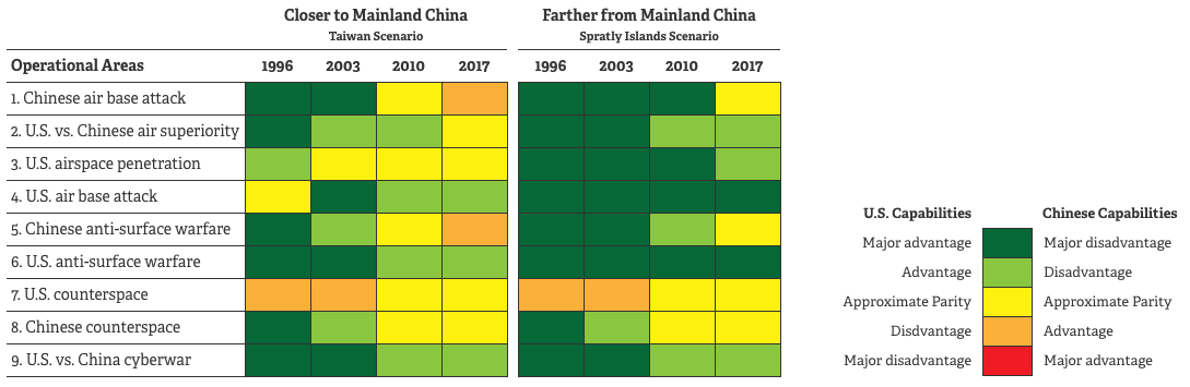 The capabilities listed in the RAND study are interesting, notable in that the air superiority category, rough parity exists as of 2017. Also, the ability to attack air bases has given an advantage to the Chinese forces.