Response to Niklas Zetterling’s Article by Christopher A. Lawrence
Mr. Zetterling is currently a professor at the Swedish War College and previously worked at the Swedish National Defense Research Establishment. As I have been having an ongoing dialogue with Prof. Zetterling on the Battle of Kursk, I have had the opportunity to witness his approach to researching historical data and the depth of research. I would recommend that all of our readers take a look at his recent article in the Journal of Slavic Military Studies entitled “Loss Rates on the Eastern Front during World War II.” Mr. Zetterling does his German research directly from the Captured German Military Records by purchasing the rolls of microfilm from the US National Archives. He is using the same German data sources that we are. Let me attempt to address his comments section by section:
The Database on Italy 1943-44:
Unfortunately, the Italian combat data was one of the early HERO research projects, with the results first published in 1971. I do not know who worked on it nor the specifics of how it was done. There are references to the Captured German Records, but significantly, they only reference division files for these battles. While I have not had the time to review Prof. Zetterling‘s review of the original research. I do know that some of our researchers have complained about parts of the Italian data. From what I’ve seen, it looks like the original HERO researchers didn’t look into the Corps and Army files, and assumed what the attached Corps artillery strengths were. Sloppy research is embarrassing, although it does occur, especially when working under severe financial constraints (for example, our Battalion-level Operations Database). If the research is sloppy or hurried, or done from secondary sources, then hopefully the errors are random, and will effectively counterbalance each other, and not change the results of the analysis. If the errors are all in one direction, then this will produce a biased result.
I have no basis to believe that Prof. Zetterling’s criticism is wrong, and do have many reasons to believe that it is correct. Until l can take the time to go through the Corps and Army files, I intend to operate under the assumption that Prof. Zetterling’s corrections are good. At some point I will need to go back through the Italian Campaign data and correct it and update the Land Warfare Database. I did compare Prof. Zetterling‘s list of battles with what was declared to be the forces involved in the battle (according to the Combat Data Subscription Service) and they show the following attached artillery:
It is clear that the battles were based on the assumption that here was Corps-level German artillery. A strength comparison between the two sides is displayed in the chart on the next page.
The Result Formula:
CEV is calculated from three factors. Therefore a consistent 20% error in casualties will result in something less than a 20% error in CEV. The mission effectiveness factor is indeed very “fuzzy,” and these is simply no systematic method or guidance in its application. Sometimes, it is not based upon the assigned mission of the unit, but its perceived mission based upon the analyst’s interpretation. But, while l have the same problems with the mission accomplishment scores as Mr. Zetterling, I do not have a good replacement. Considering the nature of warfare, I would hate to create CEVs without it. Of course, Trevor Dupuy was experimenting with creating CEVs just from casualty effectiveness, and by averaging his two CEV scores (CEVt and CEVI) he heavily weighted the CEV calculation for the TNDM towards measuring primarily casualty effectiveness (see the article in issue 5 of the Newsletter, “Numerical Adjustment of CEV Results: Averages and Means“). At this point, I would like to produce a new, single formula for CEV to replace the current two and its averaging methodology. I am open to suggestions for this.
Supply Situation:
The different ammunition usage rate of the German and US Armies is one of the reasons why adding a logistics module is high on my list of model corrections. This was discussed in Issue 2 of the Newsletter, “Developing a Logistics Model for the TNDM.” As Mr. Zetterling points out, “It is unlikely that an increase in artillery ammunition expenditure will result in a proportional increase in combat power. Rather it is more likely that there is some kind of diminished return with increased expenditure.” This parallels what l expressed in point 12 of that article: “It is suspected that this increase [in OLIs] will not be linear.”
The CEV does include “logistics.” So in effect, if one had a good logistics module, the difference in logistics would be accounted for, and the Germans (after logistics is taken into account) may indeed have a higher CEV.
General Problems with Non-Divisional Units Tooth-to-Tail Ratio
Point taken. The engagements used to test the TNDM have been gathered over a period of over 25 years, by different researchers and controlled by different management. What is counted when and where does change from one group of engagements to the next. While l do think this has not had a significant result on the model outcomes, it is “sloppy” and needs to be addressed.
The Effects of Defensive Posture
This is a very good point. If the budget was available, my first step in “redesigning” the TNDM would be to try to measure the effects of terrain on combat through the use of a large LWDB-type database and regression analysis. I have always felt that with enough engagements, one could produce reliable values for these figures based upon something other than judgement. Prof. Zetterling’s proposed methodology is also a good approach, easier to do, and more likely to get a conclusive result. I intend to add this to my list of model improvements.
Conclusions
There is one other problem with the Italian data that Prof. Zetterling did not address. This was that the Germans and the Allies had different reporting systems for casualties. Quite simply, the Germans did not report as casualties those people who were lightly wounded and treated and returned to duty from the divisional aid station. The United States and England did. This shows up when one compares the wounded to killed ratios of the various armies, with the Germans usually having in the range of 3 to 4 wounded for every one killed, while the allies tend to have 4 to 5 wounded for every one killed. Basically, when comparing the two reports, the Germans “undercount” their casualties by around 17 to 20%. Therefore, one probably needs to use a multiplier of 20 to 25% to match the two casualty systems. This was not taken into account in any the work HERO did.
Because Trevor Dupuy used three factors for measuring his CEV, this error certainly resulted in a slightly higher CEV for the Germans than should have been the case, but not a 20% increase. As Prof. Zetterling points out, the correction of the count of artillery pieces should result in a higher CEV than Col. Dupuy calculated. Finally, if Col. Dupuy overrated the value of defensive terrain, then this may result in the German CEV being slightly lower.
As you may have noted in my list of improvements (Issue 2, “Planned Improvements to the TNDM”), I did list “revalidating” to the QJM Database. [NOTE: a summary of the QJM/TNDM validation efforts can be found here.] As part of that revalidation process, we would need to review the data used in the validation data base first, account for the casualty differences in the reporting systems, and determine if the model indeed overrates the effect of terrain on defense.
Perhaps one of the most debated results of the TNDM (and its predecessors) is the conclusion that the German ground forces on average enjoyed a measurable qualitative superiority over its US and British opponents. This was largely the result of calculations on situations in Italy in 1943-44, even though further engagements have been added since the results were first presented. The calculated German superiority over the Red Army, despite the much smaller number of engagements, has not aroused as much opposition. Similarly, the calculated Israeli effectiveness superiority over its enemies seems to have surprised few.
However, there are objections to the calculations on the engagements in Italy 1943. These concern primarily the database, but there are also some questions to be raised against the way some of the calculations have been made, which may possibly have consequences for the TNDM.
Here it is suggested that the German CEV [combat effectiveness value] superiority was higher than originally calculated. There are a number of flaws in the original calculations, each of which will be discussed separately below. With the exception of one issue, all of them, if corrected, tend to give a higher German CEV.
The Database on Italy 1943-44
According to the database the German divisions had considerable fire support from GHQ artillery units. This is the only possible conclusion from the fact that several pieces of the types 15cm gun, 17cm gun, 21cm gun, and 15cm and 21cm Nebelwerfer are included in the data for individual engagements. These types of guns were almost exclusively confined to GHQ units. An example from the database are the three engagements Port of Salerno, Amphitheater, and Sele-Calore Corridor. These take place simultaneously (9-11 September 1943) with the German 16th Pz Div on the Axis side in all of them (no other division is included in the battles). Judging from the manpower figures, it seems to have been assumed that the division participated with one quarter of its strength in each of the two former battles and half its strength in the latter. According to the database, the number of guns were:
15cm gun
28
17cm gun
12
21cm gun
12
15cm NbW
27
21cm NbW
21
This would indicate that the 16th Pz Div was supported by the equivalent of more than five non-divisional artillery battalions. For the German army this is a suspiciously high number, usually there were rather something like one GHQ artillery battalion for each division, or even less. Research in the German Military Archives confirmed that the number of GHQ artillery units was far less than indicated in the HERO database. Among the useful documents found were a map showing the dispositions of 10th Army artillery units. This showed clearly that there was only one non-divisional artillery unit south of Rome at the time of the Salerno landings, the III/71 Nebelwerfer Battalion. Also the 557th Artillery Battalion (17cm gun) was present, it was included in the artillery regiment (33rd Artillery Regiment) of 15th Panzergrenadier Division during the second half of 1943. Thus the number of German artillery pieces in these engagements is exaggerated to an extent that cannot be considered insignificant. Since OLI values for artillery usually constitute a significant share of the total OLI of a force in the TNDM, errors in artillery strength cannot be dismissed easily.
While the example above is but one, further archival research has shown that the same kind of error occurs in all the engagements in September and October 1943. It has not been possible to check the engagements later during 1943, but a pattern can be recognized. The ratio between the numbers of various types of GHQ artillery pieces does not change much from battle to battle. It seems that when the database was developed, the researchers worked with the assumption that the German corps and army organizations had organic artillery, and this assumption may have been used as a “rule of thumb.” This is wrong, however; only artillery staffs, command and control units were included in the corps and army organizations, not firing units. Consequently we have a systematic error, which cannot be corrected without changing the contents of the database. It is worth emphasizing that we are discussing an exaggeration of German artillery strength of about 100%, which certainly is significant. Comparing the available archival records with the database also reveals errors in numbers of tanks and antitank guns, but these are much smaller than the errors in artillery strength. Again these errors do always inflate the German strength in those engagements l have been able to check against archival records. These errors tend to inflate German numerical strength, which of course affects CEV calculations. But there are further objections to the CEV calculations.
The Result Formula
The “result formula” weighs together three factors: casualties inflicted, distance advanced, and mission accomplishment. It seems that the first two do not raise many objections, even though the relative weight of them may always be subject to argumentation.
The third factor, mission accomplishment, is more dubious however. At first glance it may seem to be natural to include such a factor. Alter all, a combat unit is supposed to accomplish the missions given to it. However, whether a unit accomplishes its mission or not depends both on its own qualities as well as the realism of the mission assigned. Thus the mission accomplishment factor may reflect the qualities of the combat unit as well as the higher HQs and the general strategic situation. As an example, the Rapido crossing by the U.S. 36th Infantry Division can serve. The division did not accomplish its mission, but whether the mission was realistic, given the circumstances, is dubious. Similarly many German units did probably, in many situations, receive unrealistic missions, particularly during the last two years of the war (when most of the engagements in the database were fought). A more extreme example of situations in which unrealistic missions were given is the battle in Belorussia, June-July 1944, where German units were regularly given impossible missions. Possibly it is a general trend that the side which is fighting at a strategic disadvantage is more prone to give its combat units unrealistic missions.
On the other hand it is quite clear that the mission assigned may well affect both the casualty rates and advance rates. If, for example, the defender has a withdrawal mission, advance may become higher than if the mission was to defend resolutely. This must however not necessarily be handled by including a missions factor in a result formula.
I have made some tentative runs with the TNDM, testing with various CEV values to see which value produced an outcome in terms of casualties and ground gained as near as possible to the historical result. The results of these runs are very preliminary, but the tendency is that higher German CEVs produce more historical outcomes, particularly concerning combat.
Supply Situation
According to scattered information available in published literature, the U.S. artillery fired more shells per day per gun than did German artillery. In Normandy, US 155mm M1 howitzers fired 28.4 rounds per day during July, while August showed slightly lower consumption, 18 rounds per day. For the 105mm M2 howitzer the corresponding figures were 40.8 and 27.4. This can be compared to a German OKH study which, based on the experiences in Russia 1941-43, suggested that consumption of 105mm howitzer ammunition was about 13-22 rounds per gun per day, depending on the strength of the opposition encountered. For the 150mm howitzer the figures were 12-15.
While these figures should not be taken too seriously, as they are not from primary sources and they do also reflect the conditions in different theaters, they do at least indicate that it cannot be taken for granted that ammunition expenditure is proportional to the number of gun barrels. In fact there also exist further indications that Allied ammunition expenditure was greater than the German. Several German reports from Normandy indicate that they were astonished by the Allied ammunition expenditure.
It is unlikely that an increase in artillery ammunition expenditure will result in a proportional increase combat power. Rather it is more likely that there is some kind of diminished return with increased expenditure.
General Problems with Non-Divisional Units
A division usually (but not necessarily) includes various support services, such as maintenance, supply, and medical services. Non-divisional combat units have to a greater extent to rely on corps and army for such support. This makes it complicated to include such units, since when entering, for example, the manpower strength and truck strength in the TNDM, it is difficult to assess their contribution to the overall numbers.
Furthermore, the amount of such forces is not equal on the German and Allied sides. In general the Allied divisional slice was far greater than the German. In Normandy the US forces on 25 July 1944 had 812,000 men on the Continent, while the number of divisions was 18 (including the 5th Armored, which was in the process of landing on the 25th). This gives a divisional slice of 45,000 men. By comparison the German 7th Army mustered 16 divisions and 231,000 men on 1 June 1944, giving a slice of 14,437 men per division. The main explanation for the difference is the non-divisional combat units and the logistical organization to support them. In general, non-divisional combat units are composed of powerful, but supply-consuming, types like armor, artillery, antitank and antiaircraft. Thus their contribution to combat power and strain on the logistical apparatus is considerable. However I do not believe that the supporting units’ manpower and vehicles have been included in TNDM calculations.
There are however further problems with non-divisional units. While the whereabouts of tank and tank destroyer units can usually be established with sufficient certainty, artillery can be much harder to pin down to a specific division engagement. This is of course a greater problem when the geographical extent of a battle is small.
Tooth-to-Tail Ratio
Above was discussed the lack of support units in non-divisional combat units. One effect of this is to create a force with more OLI per man. This is the result of the unit‘s “tail” belonging to some other part of the military organization.
In the TNDM there is a mobility formula, which tends to favor units with many weapons and vehicles compared to the number of men. This became apparent when I was performing a great number of TNDM runs on engagements between Swedish brigades and Soviet regiments. The Soviet regiments usually contained rather few men, but still had many AFVs, artillery tubes, AT weapons, etc. The Mobility Formula in TNDM favors such units. However, I do not think this reflects any phenomenon in the real world. The Soviet penchant for lean combat units, with supply, maintenance, and other services provided by higher echelons, is not a more effective solution in general, but perhaps better suited to the particular constraints they were experiencing when forming units, training men, etc. In effect these services were existing in the Soviet army too, but formally not with the combat units.
This problem is to some extent reminiscent to how density is calculated (a problem discussed by Chris Lawrence in a recent issue of the Newsletter). It is comparatively easy to define the frontal limit of the deployment area of force, and it is relatively easy to define the lateral limits too. It is, however, much more difficult to say where the rear limit of a force is located.
When entering forces in the TNDM a rear limit is, perhaps unintentionally, drawn. But if the combat unit includes support units, the rear limit is pushed farther back compared to a force whose combat units are well separated from support units.
To what extent this affects the CEV calculations is unclear. Using the original database values, the German forces are perhaps given too high combat strength when the great number of GHQ artillery units is included. On the other hand, if the GHQ artillery units are not included, the opposite may be true.
The Effects of Defensive Posture
The posture factors are difficult to analyze, since they alone do not portray the advantages of defensive position. Such effects are also included in terrain factors.
It seems that the numerical values for these factors were assigned on the basis of professional judgement. However, when the QJM was developed, it seems that the developers did not assume the German CEV superiority. Rather, the German CEV superiority seems to have been discovered later. It is possible that the professional judgement was about as wrong on the issue of posture effects as they were on CEV. Since the British and American forces were predominantly on the offensive, while the Germans mainly defended themselves, a German CEV superiority may, at least partly, be hidden in two high effects for defensive posture.
When using corrected input data on the 20 situations in Italy September-October 1943, there is a tendency that the German CEV is higher when they attack. Such a tendency is also discernible in the engagements presented in Hitler’s Last Gamble. Appendix H, even though the number of engagements in the latter case is very small.
As it stands now this is not really more than a hypothesis, since it will take an analysis of a greater number of engagements to confirm it. However, if such an analysis is done, it must be done using several sets of data. German and Allied attacks must be analyzed separately, and preferably the data would be separated further into sets for each relevant terrain type. Since the effects of the defensive posture are intertwined with terrain factors, it is very much possible that the factors may be correct for certain terrain types, while they are wrong for others. It may also be that the factors can be different for various opponents (due to differences in training, doctrine, etc.). It is also possible that the factors are different if the forces are predominantly composed of armor units or mainly of infantry.
One further problem with the effects of defensive position is that it is probably strongly affected by the density of forces. It is likely that the main effect of the density of forces is the inability to use effectively all the forces involved. Thus it may be that this factor will not influence the outcome except when the density is comparatively high. However, what can be regarded as “high” is probably much dependent on terrain, road net quality, and the cross-country mobility of the forces.
Conclusions
While the TNDM has been criticized here, it is also fitting to praise the model. The very fact that it can be criticized in this way is a testimony to its openness. In a sense a model is also a theory, and to use Popperian terminology, the TNDM is also very testable.
It should also be emphasized that the greatest errors are probably those in the database. As previously stated, I can only conclude safely that the data on the engagements in Italy in 1943 are wrong; later engagements have not yet been checked against archival documents. Overall the errors do not represent a dramatic change in the CEV values. Rather, the Germans seem to have (in Italy 1943) a superiority on the order of 1.4-1.5, compared to an original figure of 1.2-1.3.
During September and October 1943, almost all the German divisions in southern Italy were mechanized or parachute divisions. This may have contributed to a higher German CEV. Thus it is not certain that the conclusions arrived at here are valid for German forces in general, even though this factor should not be exaggerated, since many of the German divisions in Italy were either newly raised (e.g., 26th Panzer Division) or rebuilt after the Stalingrad disaster (16th Panzer Division plus 3rd and 29th Panzergrenadier Divisions) or the Tunisian debacle (15th Panzergrenadier Division).
Allied force dispositions at the Battle of Anzio, on 1 February 1944. [U.S. Army/Wikipedia]
[The article below is reprinted from History, Numbers And War: A HERO Journal, Vol. 1, No. 1, Spring 1977, pp. 34-52]
The Lanchester Equations and Historical Warfare: An Analysis of Sixty World War II Land Engagements
By Janice B. Fain
Background and Objectives
The method by which combat losses are computed is one of the most critical parts of any combat model. The Lanchester equations, which state that a unit’s combat losses depend on the size of its opponent, are widely used for this purpose.
In addition to their use in complex dynamic simulations of warfare, the Lanchester equations have also sewed as simple mathematical models. In fact, during the last decade or so there has been an explosion of theoretical developments based on them. By now their variations and modifications are numerous, and “Lanchester theory” has become almost a separate branch of applied mathematics. However, compared with the effort devoted to theoretical developments, there has been relatively little empirical testing of the basic thesis that combat losses are related to force sizes.
One of the first empirical studies of the Lanchester equations was Engel’s classic work on the Iwo Jima campaign in which he found a reasonable fit between computed and actual U.S. casualties (Note 1). Later studies were somewhat less supportive (Notes 2 and 3), but an investigation of Korean war battles showed that, when the simulated combat units were constrained to follow the tactics of their historical counterparts, casualties during combat could be predicted to within 1 to 13 percent (Note 4).
Taken together, these various studies suggest that, while the Lanchester equations may be poor descriptors of large battles extending over periods during which the forces were not constantly in combat, they may be adequate for predicting losses while the forces are actually engaged in fighting. The purpose of the work reported here is to investigate 60 carefully selected World War II engagements. Since the durations of these battles were short (typically two to three days), it was expected that the Lanchester equations would show a closer fit than was found in studies of larger battles. In particular, one of the objectives was to repeat, in part, Willard’s work on battles of the historical past (Note 3).
The Data Base
Probably the most nearly complete and accurate collection of combat data is the data on World War II compiled by the Historical Evaluation and Research Organization (HERO). From their data HERO analysts selected, for quantitative analysis, the following 60 engagements from four major Italian campaigns:
Salerno, 9-18 Sep 1943, 9 engagements
Volturno, 12 Oct-8 Dec 1943, 20 engagements
Anzio, 22 Jan-29 Feb 1944, 11 engagements
Rome, 14 May-4 June 1944, 20 engagements
The complete data base is described in a HERO report (Note 5). The work described here is not the first analysis of these data. Statistical analyses of weapon effectiveness and the testing of a combat model (the Quantified Judgment Method, QJM) have been carried out (Note 6). The work discussed here examines these engagements from the viewpoint of the Lanchester equations to consider the question: “Are casualties during combat related to the numbers of men in the opposing forces?”
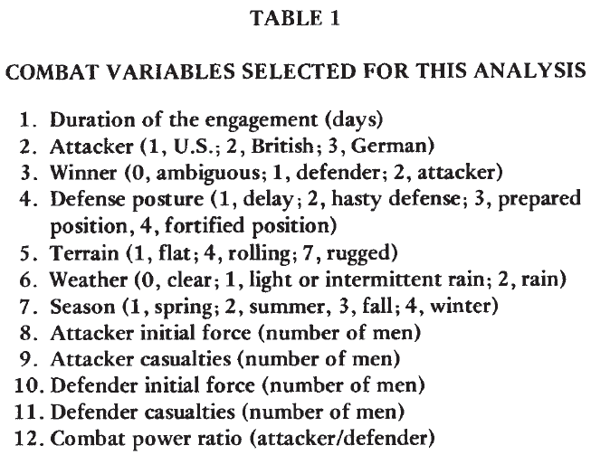
The variables chosen for this analysis are shown in Table 1. The “winners” of the engagements were specified by HERO on the basis of casualties suffered, distance advanced, and subjective estimates of the percentage of the commander’s objective achieved. Variable 12, the Combat Power Ratio, is based on the Operational Lethality Indices (OLI) of the units (Note 7).
The general characteristics of the engagements are briefly described. Of the 60, there were 19 attacks by British forces, 28 by U.S. forces, and 13 by German forces. The attacker was successful in 34 cases; the defender, in 23; and the outcomes of 3 were ambiguous. With respect to terrain, 19 engagements occurred in flat terrain; 24 in rolling, or intermediate, terrain; and 17 in rugged, or difficult, terrain. Clear weather prevailed in 40 cases; 13 engagements were fought in light or intermittent rain; and 7 in medium or heavy rain. There were 28 spring and summer engagements and 32 fall and winter engagements.
Comparison of World War II Engagements With Historical Battles
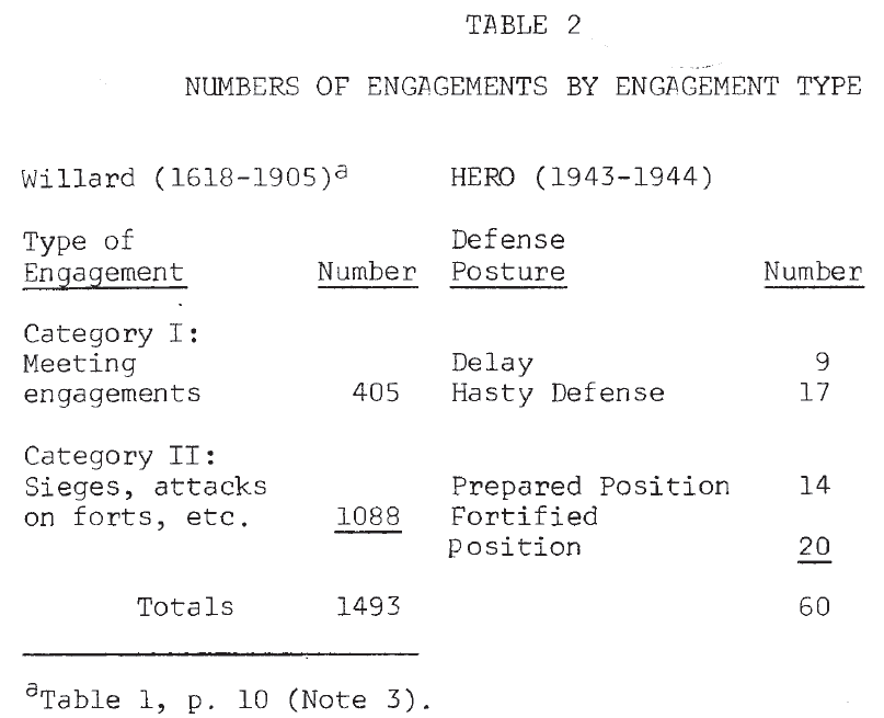
Since one purpose of this work is to repeat, in part, Willard’s analysis, comparison of these World War II engagements with the historical battles (1618-1905) studied by him will be useful. Table 2 shows a comparison of the distribution of battles by type. Willard’s cases were divided into two categories: I. meeting engagements, and II. sieges, attacks on forts, and similar operations. HERO’s World War II engagements were divided into four types based on the posture of the defender: 1. delay, 2. hasty defense, 3. prepared position, and 4. fortified position. If postures 1 and 2 are considered very roughly equivalent to Willard’s category I, then in both data sets the division into the two gross categories is approximately even.
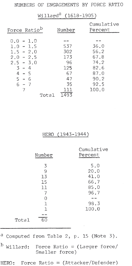
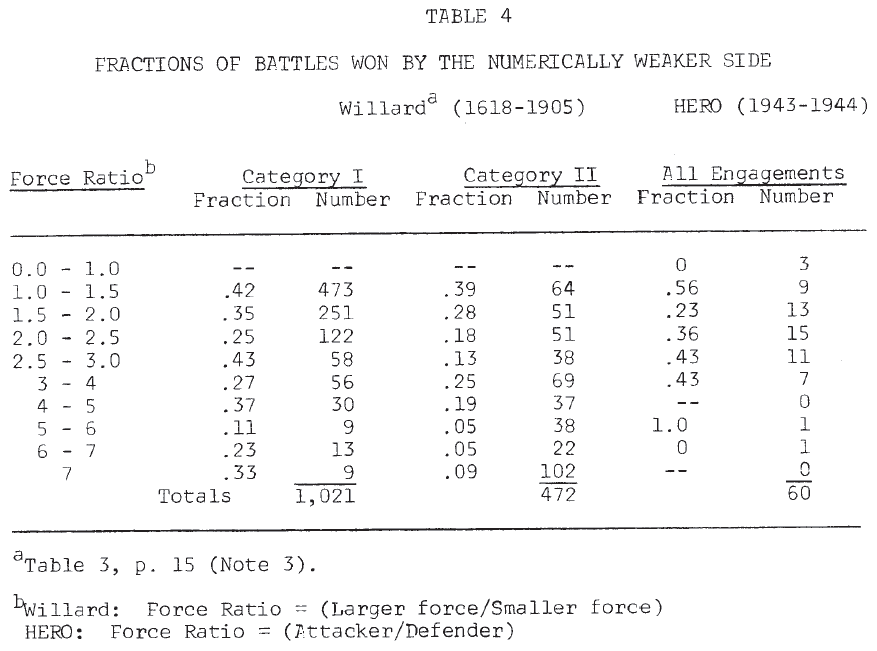
The distribution of engagements across force ratios, given in Table 3, indicated some differences. Willard’s engagements tend to cluster at the lower end of the scale (1-2) and at the higher end (4 and above), while the majority of the World War II engagements were found in mid-range (1.5 – 4) (Note 8). The frequency with which the numerically inferior force achieved victory is shown in Table 4. It is seen that in neither data set are force ratios good predictors of success in battle (Note 9).
Table 3.
Results of the Analysis Willard’s Correlation Analysis
There are two forms of the Lanchester equations. One represents the case in which firing units on both sides know the locations of their opponents and can shift their fire to a new target when a “kill” is achieved. This leads to the “square” law where the loss rate is proportional to the opponent’s size. The second form represents that situation in which only the general location of the opponent is known. This leads to the “linear” law in which the loss rate is proportional to the product of both force sizes.
As Willard points out, large battles are made up of many smaller fights. Some of these obey one law while others obey the other, so that the overall result should be a combination of the two. Starting with a general formulation of Lanchester’s equations, where g is the exponent of the target unit’s size (that is, g is 0 for the square law and 1 for the linear law), he derives the following linear equation:
log (nc/mc) = log E + g log (mo/no) (1)
where nc and mc are the casualties, E is related to the exchange ratio, and mo and no are the initial force sizes. Linear regression produces a value for g. However, instead of lying between 0 and 1, as expected, the) g‘s range from -.27 to -.87, with the majority lying around -.5. (Willard obtains several values for g by dividing his data base in various ways—by force ratio, by casualty ratio, by historical period, and so forth.) A negative g value is unpleasant. As Willard notes:
Military theorists should be disconcerted to find g < 0, for in this range the results seem to imply that if the Lanchester formulation is valid, the casualty-producing power of troops increases as they suffer casualties (Note 3).
From his results, Willard concludes that his analysis does not justify the use of Lanchester equations in large-scale situations (Note 10).
Analysis of the World War II Engagements
Willard’s computations were repeated for the HERO data set. For these engagements, regression produced a value of -.594 for g (Note 11), in striking agreement with Willard’s results. Following his reasoning would lead to the conclusion that either the Lanchester equations do not represent these engagements, or that the casualty producing power of forces increases as their size decreases.
However, since the Lanchester equations are so convenient analytically and their use is so widespread, it appeared worthwhile to reconsider this conclusion. In deriving equation (1), Willard used binomial expansions in which he retained only the leading terms. It seemed possible that the poor results might he due, in part, to this approximation. If the first two terms of these expansions are retained, the following equation results:
log (nc/mc) = log E + log (Mo-mc)/(no-nc) (2)
Repeating this regression on the basis of this equation leads to g = -.413 (Note 12), hardly an improvement over the initial results.
A second attempt was made to salvage this approach. Starting with raw OLI scores (Note 7), HERO analysts have computed “combat potentials” for both sides in these engagements, taking into account the operational factors of posture, vulnerability, and mobility; environmental factors like weather, season, and terrain; and (when the record warrants) psychological factors like troop training, morale, and the quality of leadership. Replacing the factor (mo/no) in Equation (1) by the combat power ratio produces the result) g = .466 (Note 13).
While this is an apparent improvement in the value of g, it is achieved at the expense of somewhat distorting the Lanchester concept. It does preserve the functional form of the equations, but it requires a somewhat strange definition of “killing rates.”
Analysis Based on the Differential Lanchester Equations
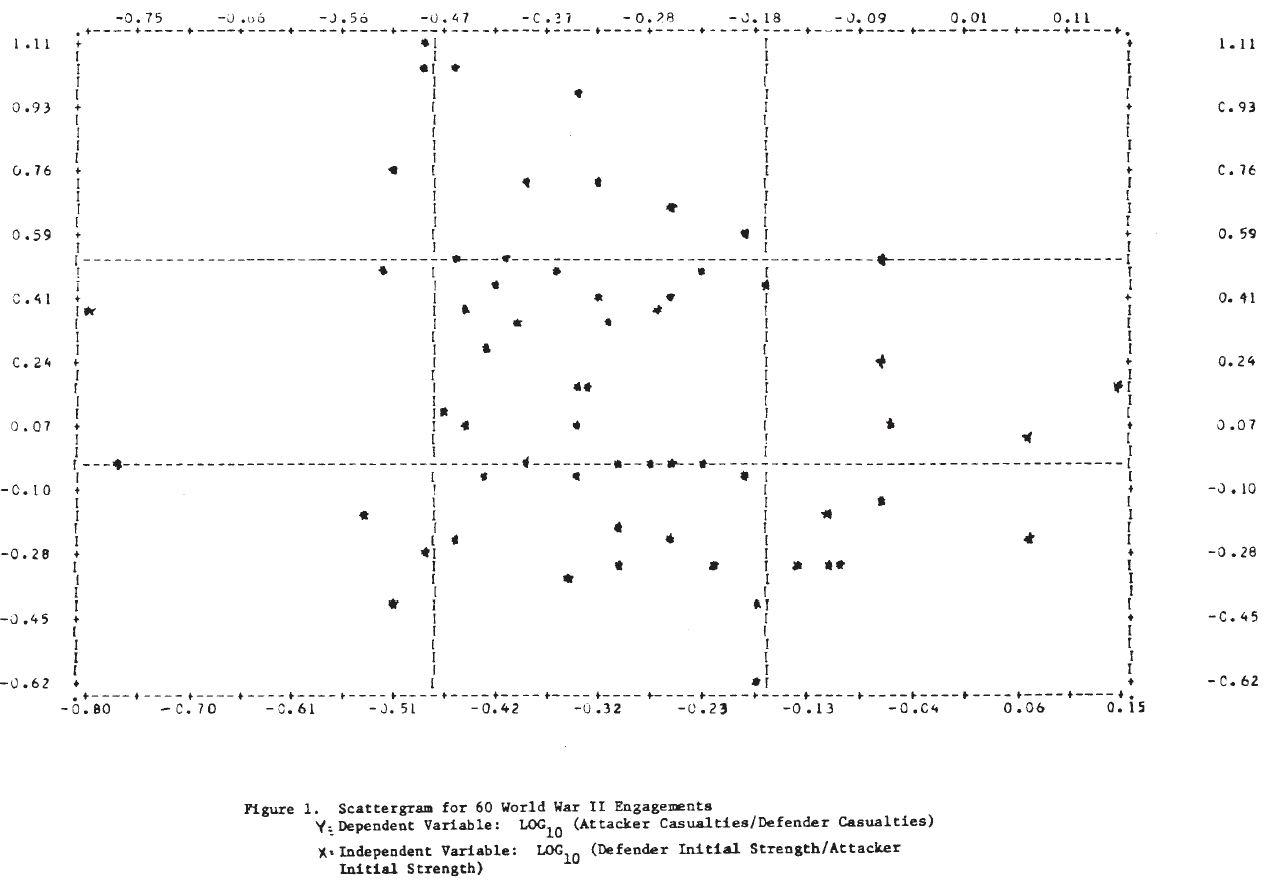
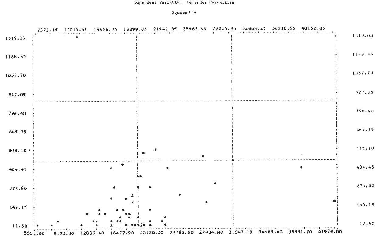
Analysis of the type carried out by Willard appears to produce very poor results for these World War II engagements. Part of the reason for this is apparent from Figure 1, which shows the scatterplot of the dependent variable, log (nc/mc), against the independent variable, log (mo/no). It is clear that no straight line will fit these data very well, and one with a positive slope would not be much worse than the “best” line found by regression. To expect the exponent to account for the wide variation in these data seems unreasonable.
Here, a simpler approach will be taken. Rather than use the data to attempt to discriminate directly between the square and the linear laws, they will be used to estimate linear coefficients under each assumption in turn, starting with the differential formulation rather than the integrated equations used by Willard.
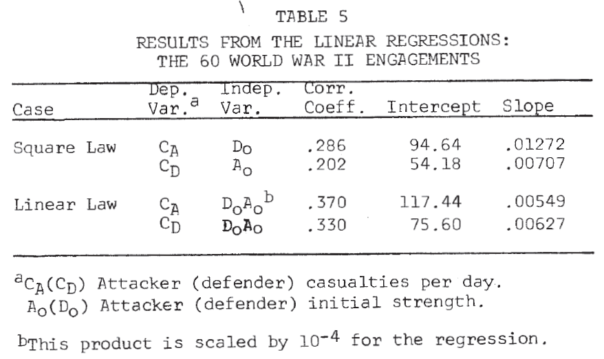
In their simplest differential form, the Lanchester equations may be written;
Square Law; dA/dt = -kdD and dD/dt = kaA (3)
Linear law: dA/dt = -k’dAD and dD/dt = k’aAD (4)
where
A(D) is the size of the attacker (defender)
dA/dt (dD/dt) is the attacker’s (defender’s) loss rate,
ka, k’a (kd, k’d) are the attacker’s (defender’s) killing rates
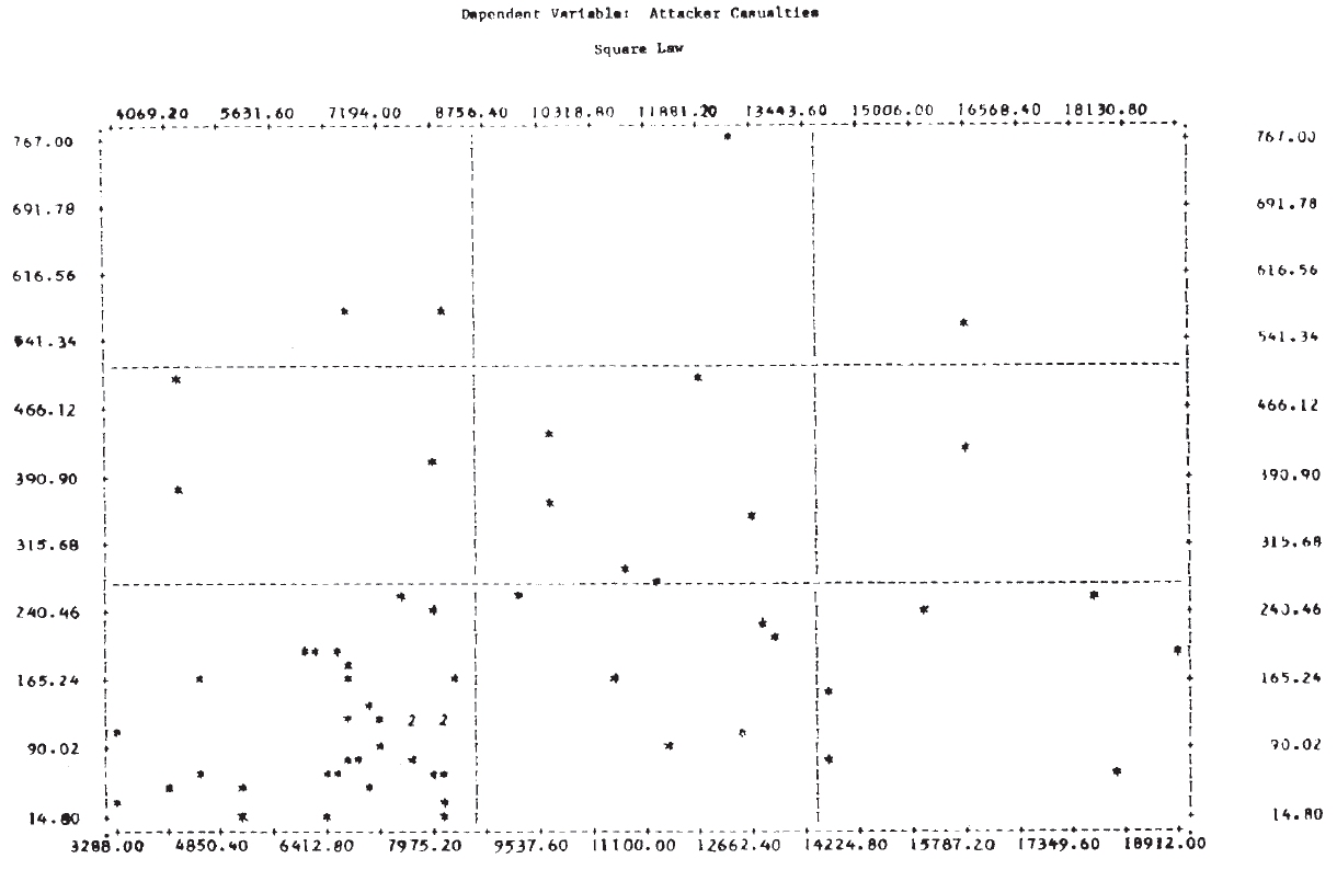
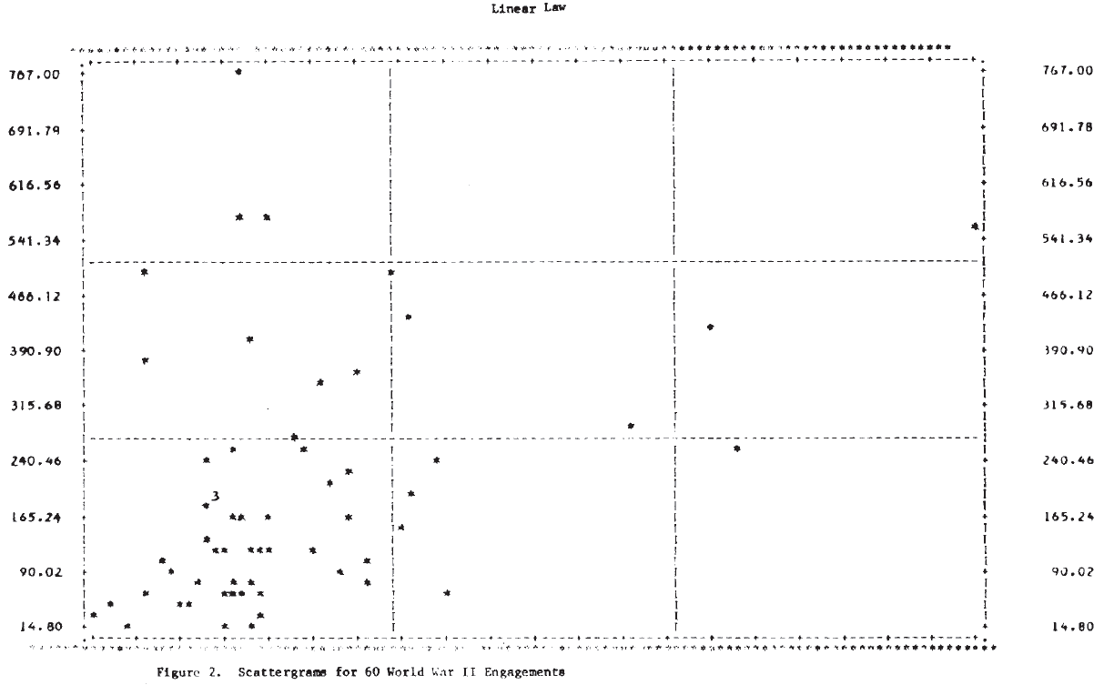
For this analysis, the day is taken as the basic time unit, and the loss rate per day is approximated by the casualties per day. Results of the linear regressions are given in Table 5. No conclusions should be drawn from the fact that the correlation coefficients are higher in the linear law case since this is expected for purely technical reasons (Note 14). A better picture of the relationships is again provided by the scatterplots in Figure 2. It is clear from these plots that, as in the case of the logarithmic forms, a single straight line will not fit the entire set of 60 engagements for either of the dependent variables.
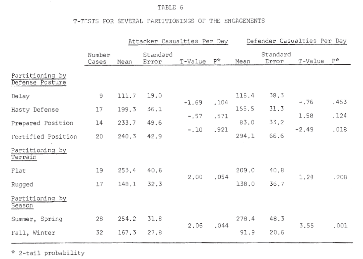
To investigate ways in which the data set might profitably be subdivided for analysis, T-tests of the means of the dependent variable were made for several partitionings of the data set. The results, shown in Table 6, suggest that dividing the engagements by defense posture might prove worthwhile.
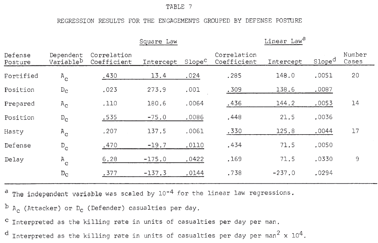
Results of the linear regressions by defense posture are shown in Table 7. For each posture, the equation that seemed to give a better fit to the data is underlined (Note 15). From this table, the following very tentative conclusions might be drawn:
In an attack on a fortified position, the attacker suffers casualties by the square law; the defender suffers casualties by the linear law. That is, the defender is aware of the attacker’s position, while the attacker knows only the general location of the defender. (This is similar to Deitchman’s guerrilla model. Note 16).
This situation is apparently reversed in the cases of attacks on prepared positions and hasty defenses.
Delaying situations seem to be treated better by the square law for both attacker and defender.
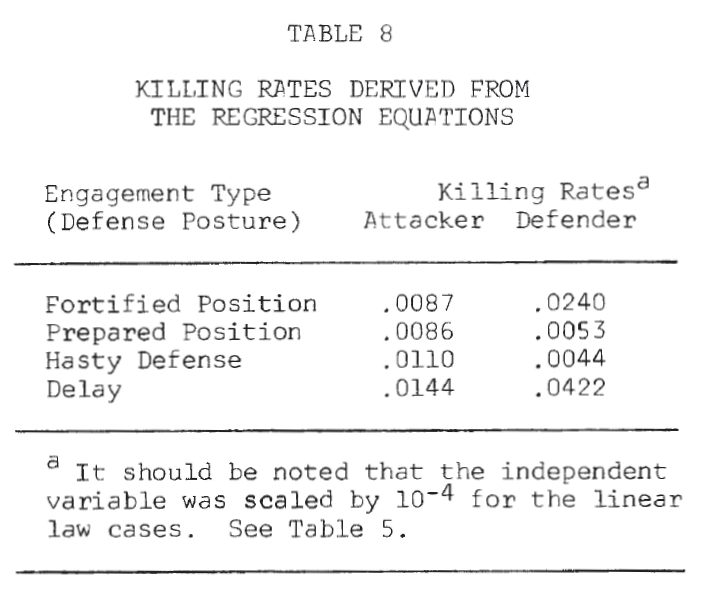
Table 8 summarizes the killing rates by defense posture. The defender has a much higher killing rate than the attacker (almost 3 to 1) in a fortified position. In a prepared position and hasty defense, the attacker appears to have the advantage. However, in a delaying action, the defender’s killing rate is again greater than the attacker’s (Note 17).
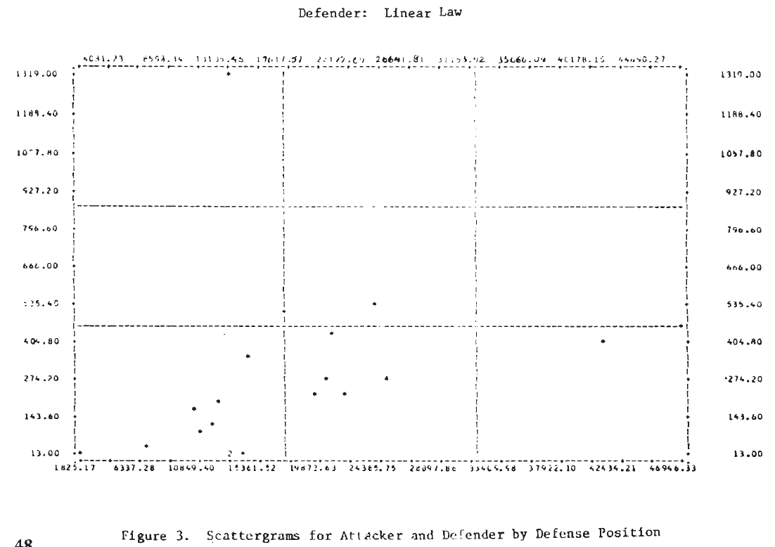
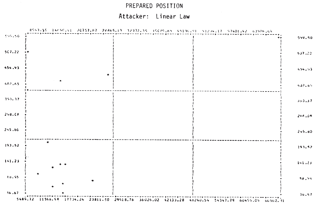
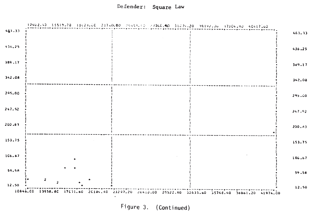
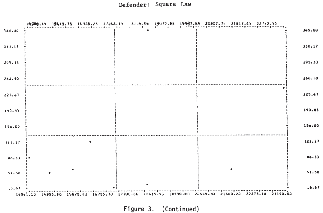
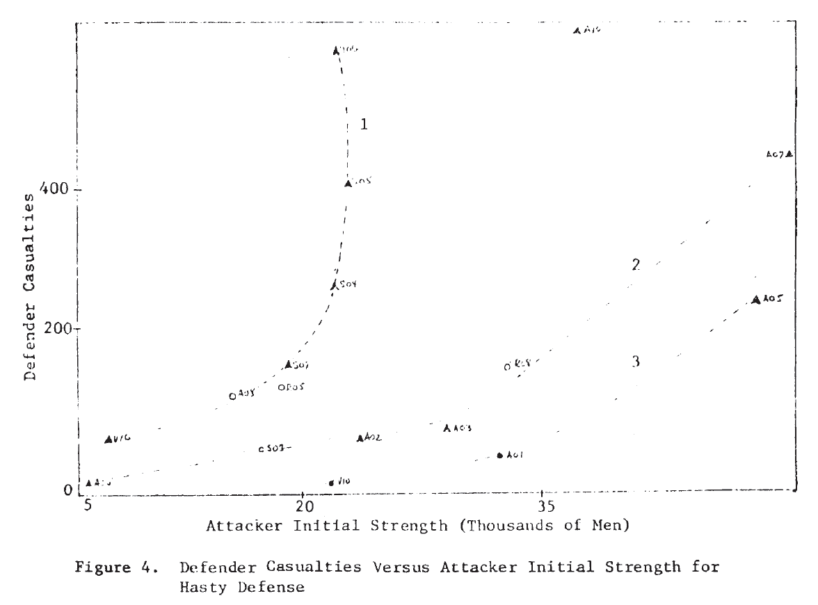
Figure 3 shows the scatterplots for these cases. Examination of these plots suggests that a tentative answer to the study question posed above might be: “Yes, casualties do appear to be related to the force sizes, but the relationship may not be a simple linear one.”
In several of these plots it appears that two or more functional forms may be involved. Consider, for example, the defender‘s casualties as a function of the attacker’s initial strength in the case of a hasty defense. This plot is repeated in Figure 4, where the points appear to fit the curves sketched there. It would appear that there are at least two, possibly three, separate relationships. Also on that plot, the individual engagements have been identified, and it is interesting to note that on the curve marked (1), five of the seven attacks were made by Germans—four of them from the Salerno campaign. It would appear from this that German attacks are associated with higher than average defender casualties for the attacking force size. Since there are so few data points, this cannot be more than a hint or interesting suggestion.
Future Research
This work suggests two conclusions that might have an impact on future lines of research on combat dynamics:
Tactics appear to be an important determinant of combat results. This conclusion, in itself, does not appear startling, at least not to the military. However, it does not always seem to have been the case that tactical questions have been considered seriously by analysts in their studies of the effects of varying force levels and force mixes.
Historical data of this type offer rich opportunities for studying the effects of tactics. For example, consideration of the narrative accounts of these battles might permit re-coding the engagements into a larger, more sensitive set of engagement categories. (It would, of course, then be highly desirable to add more engagements to the data set.)
While predictions of the future are always dangerous, I would nevertheless like to suggest what appears to be a possible trend. While military analysis of the past two decades has focused almost exclusively on the hardware of weapons systems, at least part of our future analysis will be devoted to the more behavioral aspects of combat.
Janice Bloom Fain, a Senior Associate of CACI, lnc., is a physicist whose special interests are in the applications of computer simulation techniques to industrial and military operations; she is the author of numerous reports and articles in this field. This paper was presented by Dr. Fain at the Military Operations Research Symposium at Fort Eustis, Virginia.
[5.] HERO, “A Study of the Relationship of Tactical Air Support Operations to Land Combat, Appendix B, Historical Data Base.” Historical Evaluation and Research Organization, report prepared for the Defense Operational Analysis Establishment, U.K.T.S.D., Contract D-4052 (1971).
[6.] T. N. Dupuy, The Quantified Judgment Method of Analysis of Historical Combat Data, HERO Monograph, (January 1973); HERO, “Statistical Inference in Analysis in Combat,” Annex F, Historical Data Research on Tactical Air Operations, prepared for Headquarters USAF, Assistant Chief of Staff for Studies and Analysis, Contract No. F-44620-70-C-0058 (1972).
[7.] The Operational Lethality Index (OLI) is a measure of weapon effectiveness developed by HERO.
[8.] Since Willard’s data did not indicate which side was the attacker, his force ratio is defined to be (larger force/smaller force). The HERO force ratio is (attacker/defender).
[9.] Since the criteria for success may have been rather different for the two sets of battles, this comparison may not be very meaningful.
[10.] This work includes more complex analysis in which the possibility that the two forces may be engaging in different types of combat is considered, leading to the use of two exponents rather than the single one, Stochastic combat processes are also treated.
[11.] Correlation coefficient = -.262;
Intercept = .00115; slope = -.594.
[12.] Correlation coefficient = -.184;
Intercept = .0539; slope = -,413.
[13.] Correlation coefficient = .303;
Intercept = -.638; slope = .466.
[14.] Correlation coefficients for the linear law are inflated with respect to the square law since the independent variable is a product of force sizes and, thus, has a higher variance than the single force size unit in the square law case.
[15.] This is a subjective judgment based on the following considerations Since the correlation coefficient is inflated for the linear law, when it is lower the square law case is chosen. When the linear law correlation coefficient is higher, the case with the intercept closer to 0 is chosen.
[17.] As pointed out by Mr. Alan Washburn, who prepared a critique on this paper, when comparing numerical values of the square law and linear law killing rates, the differences in units must be considered. (See footnotes to Table 7).
Today’s edition of TDI Friday Read asks the question, how do we know if the theories and concepts we use to understand and explain war and warfare accurately depict reality? There is certainly no shortage of explanatory theories available, starting with Sun Tzu in the 6th century BCE and running to the present. As I have mentioned before, all combat models and simulations are theories about how combat works. Military doctrine is also a functional theory of warfare. But how do we know if any of these theories are actually true?
Well, one simple way to find out if a particular theory is valid is to use it to predict the outcome of the phenomenon it purports to explain. Testing theory through prediction is a fundamental aspect of the philosophy of science. If a theory is accurate, it should be able to produce a reasonable accurate prediction of future behavior.
In his 2016 article, “Can We Predict Politics? Toward What End?” Michael D. Ward, a Professor of Political Science at Duke University, made a case for a robust effort for using prediction as a way of evaluating the thicket of theory populating security and strategic studies. Dropping invalid theories and concepts is important, but there is probably more value in figuring out how and why they are wrong.
Trevor Dupuy and TDI publicly put their theories to the test in the form of combat casualty estimates for the 1991 Gulf Way, the U.S. intervention in Bosnia, and the Iraqi insurgency. How well did they do?
Dupuy himself argued passionately for independent testing of combat models against real-world data, a process known as validation. This is actually seldom done in the U.S. military operations research community.
However, TDI has done validation testing of Dupuy’s Quantified Judgement Model (QJM) and Tactical Numerical Deterministic Model (TNDM). The results are available for all to judge.
I will conclude this post on a dissenting note. Trevor Dupuy spent decades arguing for more rigor in the development of combat models and analysis, with only modest success. In fact, he encountered significant skepticism and resistance to his ideas and proposals. To this day, the U.S. Defense Department seems relatively uninterested in evidence-based research on this subject. Why?
David Wilkinson, Editor-in-Chief of the Oxford Review, wrote a fascinating blog post looking at why practitioners seem to have little actual interest in evidence-based practice.
The problem with evidence based practice is that outside of areas like health care and aviation/technology is that most people in organisations don’t care about having research evidence for almost anything they do. That doesn’t mean they are not interesting in research but they are just not that interested in using the research to change how they do things – period.
His explanation for why this is and what might be done to remedy the situation is quite interesting.
Due to their elegant simplicity, U.S. military operations researchers nevertheless began incorporating the Lanchester equations into their land warfare computer combat models and simulations in the 1950s and 60s. The equations are the basis for many models and simulations used throughout the U.S. defense community today.
The problem with using Lanchester’s equations is that, despite numerous efforts, no one has been able to demonstrate that they accurately represent real-world combat.
Trevor Dupuy was critical of combat models based on the Lanchester equations because they cannot account for the role behavioral and moral (i.e. human) factors play in combat.
He was also critical of models and simulations that had not been tested to see whether they could reliably represent real-world combat experience. In the modeling and simulation community, this sort of testing is known as validation.
The use of unvalidated concepts, like the Lanchester equations, and unvalidated combat models and simulations persists. Critics have dubbed this the “base of sand” problem, and it continues to affect not only models and simulations, but all abstract theories of combat, including those represented in military doctrine.
After its initial development using a 60-engagement WWII database, the QJM was tested in 1973 by application of its relationships and factors to a validation database of 21 World War II engagements in Northwest Europe in 1944 and 1945. The original model proved to be 95% accurate in explaining the outcomes of these additional engagements. Overall accuracy in predicting the results of the 81 engagements in the developmental and validation databases was 93%.[1]
During the same period the QJM was converted from a static model that only predicted success or failure to one capable of also predicting attrition and movement. This was accomplished by adding variables and modifying factor values. The original QJM structure was not changed in this process. The addition of movement and attrition as outputs allowed the model to be used dynamically in successive “snapshot” iterations of the same engagement.
From 1973 to 1979 the QJM’s formulae, procedures, and variable factor values were tested against the results of all of the 52 significant engagements of the 1967 and 1973 Arab-Israeli Wars (19 from the former, 33 from the latter). The QJM was able to replicate all of those engagements with an accuracy of more than 90%?[2]
In 1979 the improved QJM was revalidated by application to 66 engagements. These included 35 from the original 81 engagements (the “development database”), and 31 new engagements. The new engagements included five from World War II and 26 from the 1973 Middle East War. This new validation test considered four outputs: success/failure, movement rates, personnel casualties, and tank losses. The QJM predicted success/failure correctly for about 85% of the engagements. It predicted movement rates with an error of 15% and personnel attrition with an error of 40% or less. While the error rate for tank losses was about 80%, it was discovered that the model consistently underestimated tank losses because input data included all kinds of armored vehicles, but output data losses included only numbers of tanks.[3]
This completed the original validations efforts of the QJM. The data used for the validations, and parts of the results of the validation, were published, but no formal validation report was issued. The validation was conducted in-house by Colonel Dupuy’s organization, HERO [Historical Evaluation Research Organization]. The data used were mostly from division-level engagements, although they included some corps- and brigade-level actions. We count these as two separate validation efforts.
The Development of the TNDM and Desert Storm
In 1990 Col. Dupuy, with the collaborative assistance of Dr. James G. Taylor (author of Lanchester Models of Warfare [vol. 1] [vol. 2], published by the Operations Research Society of America, Arlington, Virginia, in 1983) introduced a significant modification: the representation of the passage of time in the model. Instead of resorting to successive “snapshots,” the introduction of Taylor’s differential equation technique permitted the representation of time as a continuous flow. While this new approach required substantial changes to the software, the relationship of the model to historical experience was unchanged.[4] This revision of the model also included the substitution of formulae for some of its tables so that there was a continuous flow of values across the individual points in the tables. It also included some adjustment to the values and tables in the QJM. Finally, it incorporated a revised OLI [Operational Lethality Index] calculation methodology for modem armor (mobile fighting machines) to take into account all the factors that influence modern tank warfare.[5] The model was reprogrammed in Turbo PASCAL (the original had been written in BASIC). The new model was called the TNDM (Tactical Numerical Deterministic Model).
Also, in 1990, Trevor Dupuy published an abbreviated form of the TNDM in the book Attrition: Forecasting Battle Casualties and Equipment Losses in Modern War. A brief validation exercise using 12 battles from 1805 to 1973 was published in this book.[7] This version was used for creation of M-COAT[8] and was also separately tested by a student (Lieutenant Gozel) at the Naval Postgraduate School in 2000.[9] This version did not have the firepower scoring system, and as such neither M-COAT, Lieutenant Gozel’s test, nor Colonel Dupuy’s 12-battle validation included the OLI methodology that is in the primary version of the TNDM.
For counting purposes, I consider the Gulf War the third validation of the model. In the end, for any model, the proof is in the pudding. Can the model be used as a predictive tool or not? If not, then there is probably a fundamental flaw or two in the model. Still the validation of the TNDM was somewhat second-hand, in the sense that the closely-related previous model, the QJM, was validated in the 1970s to 200 World War II and 1967 and 1973 Arab-Israeli War battles, but the TNDM had not been. Clearly, something further needed to be done.
The Battalion-Level Validation of the TNDM
Under the guidance of Christopher A. Lawrence, The Dupuy Institute undertook a battalion-level validation of the TNDM in late 1996. This effort tested the model against 76 engagements from World War I, World War II, and the post-1945 world including Vietnam, the Arab-Israeli Wars, the Falklands War, Angola, Nicaragua, etc. This effort was thoroughly documented in The International TNDM Newsletter.[10] This effort was probably one of the more independent and better-documented validations of a casualty estimation methodology that has ever been conducted to date, in that:
The data was independently assembled (assembled for other purposes before the validation) by a number of different historians.
There were no calibration runs or adjustments made to the model before the test.
The data included a wide range of material from different conflicts and times (from 1918 to 1983).
The validation runs were conducted independently (Susan Rich conducted the validation runs, while Christopher A. Lawrence evaluated them).
The results of the validation were fully published.
The people conducting the validation were independent, in the sense that:
a) there was no contract, management, or agency requesting the validation;
b) none of the validators had previously been involved in designing the model, and had only very limited experience in using it; and
c) the original model designer was not able to oversee or influence the validation.[11]
The validation was not truly independent, as the model tested was a commercial product of The Dupuy Institute, and the person conducting the test was an employee of the Institute. On the other hand, this was an independent effort in the sense that the effort was employee-initiated and not requested or reviewed by the management of the Institute. Furthermore, the results were published.
The TNDM was also given a limited validation test back to its original WWII data around 1997 by Niklas Zetterling of the Swedish War College, who retested the model to about 15 or so Italian campaign engagements. This effort included a complete review of the historical data used for the validation back to their primarily sources, and details were published in The International TNDM Newsletter.[12]
There has been one other effort to correlate outputs from QJM/TNDM-inspired formulae to historical data using the Ardennes and Kursk campaign-level (i.e., division-level) databases.[13] This effort did not use the complete model, but only selective pieces of it, and achieved various degrees of “goodness of fit.” While the model is hypothetically designed for use from squad level to army group level, to date no validation has been attempted below battalion level, or above division level. At this time, the TNDM also needs to be revalidated back to its original WWII and Arab-Israeli War data, as it has evolved since the original validation effort.
The Corps- and Division-level Validations of the TNDM
Having now having done one extensive battalion-level validation of the model and published the results in our newsletters, Volume 1, issues 5 and 6, we were then presented an opportunity in 2006 to conduct two more validations of the model. These are discussed in depth in two articles of this issue of the newsletter.
These validations were again conducted using historical data, 24 days of corps-level combat and 25 cases of division-level combat drawn from the Battle of Kursk during 4-15 July 1943. It was conducted using an independently-researched data collection (although the research was conducted by The Dupuy Institute), using a different person to conduct the model runs (although that person was an employee of the Institute) and using another person to compile the results (also an employee of the Institute). To summarize the results of this validation (the historical figure is listed first followed by the predicted result):
There was one other effort that was done as part of work we did for the Army Medical Department (AMEDD). This is fully explained in our report Casualty Estimation Methodologies Study: The Interim Report dated 25 July 2005. In this case, we tested six different casualty estimation methodologies to 22 cases. These consisted of 12 division-level cases from the Italian Campaign (4 where the attack failed, 4 where the attacker advanced, and 4 Where the defender was penetrated) and 10 cases from the Battle of Kursk (2 cases Where the attack failed, 4 where the attacker advanced and 4 where the defender was penetrated). These 22 cases were randomly selected from our earlier 628 case version of the DLEDB (Division-level Engagement Database; it now has 752 cases). Again, the TNDM performed as well as or better than any of the other casualty estimation methodologies tested. As this validation effort was using the Italian engagements previously used for validation (although some had been revised due to additional research) and three of the Kursk engagements that were later used for our division-level validation, then it is debatable whether one would want to call this a seventh validation effort. Still, it was done as above with one person assembling the historical data and another person conducting the model runs. This effort was conducted a year before the corps and division-level validation conducted above and influenced it to the extent that we chose a higher CEV (Combat Effectiveness Value) for the later validation. A CEV of 2.5 was used for the Soviets for this test, vice the CEV of 3.0 that was used for the later tests.
Summation
The QJM has been validated at least twice. The TNDM has been tested or validated at least four times, once to an upcoming, imminent war, once to battalion-level data from 1918 to 1989, once to division-level data from 1943 and once to corps-level data from 1943. These last four validation efforts have been published and described in depth. The model continues, regardless of which validation is examined, to accurately predict outcomes and make reasonable predictions of advance rates, loss rates and armor loss rates. This is regardless of level of combat (battalion, division or corps), historic period (WWI, WWII or modem), the situation of the combats, or the nationalities involved (American, German, Soviet, Israeli, various Arab armies, etc.). As the QJM, the model was effectively validated to around 200 World War II and 1967 and 1973 Arab-Israeli War battles. As the TNDM, the model was validated to 125 corps-, division-, and battalion-level engagements from 1918 to 1989 and used as a predictive model for the 1991 Gulf War. This is the most extensive and systematic validation effort yet done for any combat model. The model has been tested and re-tested. It has been tested across multiple levels of combat and in a wide range of environments. It has been tested where human factors are lopsided, and where human factors are roughly equal. It has been independently spot-checked several times by others outside of the Institute. It is hard to say what more can be done to establish its validity and accuracy.
NOTES
[1] It is unclear what these percentages, quoted from Dupuy in the TNDM General Theoretical Description, specify. We suspect it is a measurement of the model’s ability to predict winner and loser. No validation report based on this effort was ever published. Also, the validation figures seem to reflect the results after any corrections made to the model based upon these tests. It does appear that the division-level validation was “incremental.” We do not know if the earlier validation tests were tested back to the earlier data, but we have reason to suspect not.
[2] The original QJM validation data was first published in the Combat Data Subscription Service Supplement, vol. 1, no. 3 (Dunn Loring VA: HERO, Summer 1975). (HERO Report #50) That effort used data from 1943 through 1973.
[3] HERO published its QJM validation database in The QJM Data Base (3 volumes) Fairfax VA: HERO, 1985 (HERO Report #100).
[5] This had the unfortunate effect of undervaluing WWII-era armor by about 75% relative to other WWII weapons when modeling WWII engagements. This left The Dupuy Institute with the compromise methodology of using the old OLI method for calculating armor (Mobile Fighting Machines) when doing WWII engagements and using the new OLI method for calculating armor when doing modem engagements
[6] Testimony of Col. T. N. Dupuy, USA, Ret, Before the House Armed Services Committee, 13 Dec 1990. The Dupuy InstituteFile I-30, “Iraqi Invasion of Kuwait.”
[8] M-COAT is the Medical Course of Action Tool created by Major Bruce Shahbaz. It is a spreadsheet model based upon the elements of the TNDM provided in Dupuy’s Attrition (op. cit.) It used a scoring system derived from elsewhere in the U.S. Army. As such, it is a simplified form of the TNDM with a different weapon scoring system.
[10] Lawrence, Christopher A. “Validation of the TNDM at Battalion Level.” The International TNDM Newsletter, vol. 1, no. 2 (October 1996); Bongard, Dave “The 76 Battalion-Level Engagements.” The International TNDM Newsletter, vol. 1, no. 4 (February 1997); Lawrence, Christopher A. “The First Test of the TNDM Battalion-Level Validations: Predicting the Winner” and “The Second Test of the TNDM Battalion-Level Validations: Predicting Casualties,” The International TNDM Newsletter, vol. 1 no. 5 (April 1997); and Lawrence, Christopher A. “Use of Armor in the 76 Battalion-Level Engagements,” and “The Second Test of the Battalion-Level Validation: Predicting Casualties Final Scorecard.” The International TNDM Newsletter, vol. 1, no. 6 (June 1997).
[11] Trevor N. Dupuy passed away in July 1995, and the validation was conducted in 1996 and 1997.
[12] Zetterling, Niklas. “CEV Calculations in Italy, 1943,” The International TNDM Newsletter, vol. 1, no. 6. McLean VA: The Dupuy Institute, June 1997. See also Research Plan, The Dupuy InstituteReport E-3, McLean VA: The Dupuy Institute, 7 Oct 1998.
[13] See Gözel, “Fitting Firepower Score Models to the Battle of Kursk Data.”
Soldiers from Britain’s Royal Artillery train in a “virtual world” during Exercise Steel Sabre, 2015 [Sgt Si Longworth RLC (Phot)/MOD]
Military History and Validation of Combat Models
A Presentation at MORS Mini-Symposium on Validation, 16 Oct 1990
By Trevor N. Dupuy
In the operations research community there is some confusion as to the respective meanings of the words “validation” and “verification.” My definition of validation is as follows:
“To confirm or prove that the output or outputs of a model are consistent with the real-world functioning or operation of the process, procedure, or activity which the model is intended to represent or replicate.”
In this paper the word “validation” with respect to combat models is assumed to mean assurance that a model realistically and reliably represents the real world of combat. Or, in other words, given a set of inputs which reflect the anticipated forces and weapons in a combat encounter between two opponents under a given set of circumstances, the model is validated if we can demonstrate that its outputs are likely to represent what would actually happen in a real-world encounter between these forces under those circumstances
Thus, in this paper, the word “validation” has nothing to do with the correctness of computer code, or the apparent internal consistency or logic of relationships of model components, or with the soundness of the mathematical relationships or algorithms, or with satisfying the military judgment or experience of one individual.
True validation of combat models is not possible without testing them against modern historical combat experience. And so, in my opinion, a model is validated only when it will consistently replicate a number of military history battle outcomes in terms of: (a) Success-failure; (b) Attrition rates; and (c) Advance rates.
“Why,” you may ask, “use imprecise, doubtful, and outdated history to validate a modem, scientific process? Field tests, experiments, and field exercises can provide data that is often instrumented, and certainly more reliable than any historical data.”
I recognize that military history is imprecise; it is only an approximate, often biased and/or distorted, and frequently inconsistent reflection of what actually happened on historical battlefields. Records are contradictory. I also recognize that there is an element of chance or randomness in human combat which can produce different results in otherwise apparently identical circumstances. I further recognize that history is retrospective, telling us only what has happened in the past. It cannot predict, if only because combat in the future will be fought with different weapons and equipment than were used in historical combat.
Despite these undoubted problems, military history provides more, and more accurate information about the real world of combat, and how human beings behave and perform under varying circumstances of combat, than is possible to derive or compile from arty other source. Despite some discrepancies, patterns are unmistakable and consistent. There is always a logical explanation for any individual deviations from the patterns. Historical examples that are inconsistent, or that are counter-intuitive, must be viewed with suspicion as possibly being poor or false history.
Of course absolute prediction of a future event is practically impossible, although not necessarily so theoretically. Any speculations which we make from tests or experiments must have some basis in terms of projections from past experience.
Training or demonstration exercises, proving ground tests, field experiments, all lack the one most pervasive and most important component of combat: Fear in a lethal environment. There is no way in peacetime, or non-battlefield, exercises, test, or experiments to be sure that the results are consistent with what would have been the behavior or performance of individuals or units or formations facing hostile firepower on a real battlefield.
We know from the writings of the ancients (for instance Sun Tze—pronounced Sun Dzuh—and Thucydides) that have survived to this day that human nature has not changed since the dawn of history. The human factor the way in which humans respond to stimuli or circumstances is the most important basis for speculation and prediction. What about the “scientific” approach of those who insist that we cart have no confidence in the accuracy or reliability of historical data, that it is therefore unscientific, and therefore that it should be ignored? These people insist that only “scientific” data should be used in modeling.
In fact, every model is based upon fundamental assumptions that are intuitive and unprovable. The first step in the creation of a model is a step away from scientific reality in seeking a basis for an unreal representation of a real phenomenon. I have shown that the unreality is perpetuated when we use other imitations of reality as the basis for representing reality. History is less than perfect, but to ignore it, and to use only data that is bound to be wrong, assures that we will not be able to represent human behavior in real combat.
At the risk of repetition, and even of protesting too much, let me assure you that I am well aware of the shortcomings of military history:
The record which is available to us, which is history, only approximately reflects what actually happened. It is incomplete. It is often biased, it is often distorted. Even when it is accurate, it may be reflecting chance rather than normal processes. It is neither precise nor consistent. But, it provides more, and more accurate, information on the real world of battle than is available from the most thoroughly documented field exercises, proving ground less, or laboratory or field experiments.
Military history is imperfect. At best it reflects the actions and interactions of unpredictable human beings. We must always realize that a single historical example can be misleading for either of two reasons: (1) The data may be inaccurate, or (2) The data may be accurate, but untypical.
Nevertheless, history is indispensable. I repeat that the most pervasive characteristic of combat is fear in a lethal environment. For all of its imperfections, military history and only military history represents what happens under the environmental condition of fear.
Unfortunately, and somewhat unfairly, the reported findings of S.L.A. Marshall about human behavior in combat, which he reported in Men Against Fire, have been recently discounted by revisionist historians who assert that he never could have physically performed the research on which the book’s findings were supposedly based. This has raised doubts about Marshall’s assertion that 85% of infantry soldiers didn’t fire their weapons in combat in World War ll. That dramatic and surprising assertion was first challenged in a New Zealand study which found, on the basis of painstaking interviews, that most New Zealanders fired their weapons in combat. Thus, either Americans were different from New Zealanders, or Marshall was wrong. And now American historians have demonstrated that Marshall had had neither the time nor the opportunity to conduct his battlefield interviews which he claimed were the basis for his findings.
I knew Marshall, moderately well. I was fully as aware of his weaknesses as of his strengths. He was not a historian. I deplored the imprecision and lack of documentation in Men Against Fire. But the revisionist historians have underestimated the shrewd journalistic assessment capability of “SLAM” Marshall. His observations may not have been scientifically precise, but they were generally sound, and his assessment has been shared by many American infantry officers whose judgements l also respect. As to the New Zealand study, how many people will, after the war, admit that they didn’t fire their weapons?
Perhaps most important, however, in judging the assessments of SLAM Marshall, is a recent study by a highly-respected British operations research analyst, David Rowland. Using impeccable OR methods Rowland has demonstrated that Marshall’s assessment of the inefficient performance, or non-performance, of most soldiers in combat was essentially correct. An unclassified version of Rowland’s study, “Assessments of Combat Degradation,” appeared in the June 1986 issue of the Royal United Services Institution Journal.
Rowland was led to his investigations by the fact that soldier performance in field training exercises, using the British version of MILES technology, was not consistent with historical experience. Even after allowances for degradation from theoretical proving ground capability of weapons, defensive rifle fire almost invariably stopped any attack in these field trials. But history showed that attacks were often in fact, usually successful. He therefore began a study in which he made both imaginative and scientific use of historical data from over 100 small unit battles in the Boer War and the two World Wars. He demonstrated that when troops are under fire in actual combat, there is an additional degradation of performance by a factor ranging between 10 and 7. A degradation virtually of an order of magnitude! And this, mind you, on top of a comparable built-in degradation to allow for the difference between field conditions and proving ground conditions.
Not only does Rowland‘s study corroborate SLAM Marshall’s observations, it showed conclusively that field exercises, training competitions and demonstrations, give results so different from real battlefield performance as to render them useless for validation purposes.
Which brings us back to military history. For all of the imprecision, internal contradictions, and inaccuracies inherent in historical data, at worst the deviations are generally far less than a factor of 2.0. This is at least four times more reliable than field test or exercise results.
I do not believe that history can ever repeat itself. The conditions of an event at one time can never be precisely duplicated later. But, bolstered by the Rowland study, I am confident that history paraphrases itself.
If large bodies of historical data are compiled, the patterns are clear and unmistakable, even if slightly fuzzy around the edges. Behavior in accordance with this pattern is therefore typical. As we have already agreed, sometimes behavior can be different from the pattern, but we know that it is untypical, and we can then seek for the reason, which invariably can be discovered.
This permits what l call an actuarial approach to data analysis. We can never predict precisely what will happen under any circumstances. But the actuarial approach, with ample data, provides confidence that the patterns reveal what is to happen under those circumstances, even if the actual results in individual instances vary to some extent from this “norm” (to use the Soviet military historical expression.).
It is relatively easy to take into account the differences in performance resulting from new weapons and equipment. The characteristics of the historical weapons and the current (or projected) weapons can be readily compared, and adjustments made accordingly in the validation procedure.
In the early 1960s an effort was made at SHAPE Headquarters to test the ATLAS Model against World War II data for the German invasion of Western Europe in May, 1940. The first excursion had the Allies ending up on the Rhine River. This was apparently quite reasonable: the Allies substantially outnumbered the Germans, they had more tanks, and their tanks were better. However, despite these Allied advantages, the actual events in 1940 had not matched what ATLAS was now predicting. So the analysts did a little “fine tuning,” (a splendid term for fudging). Alter the so-called adjustments, they tried again, and ran another excursion. This time the model had the Allies ending up in Berlin. The analysts (may the Lord forgive them!) were quite satisfied with the ability of ATLAS to represent modem combat. (Or at least they said so.) Their official conclusion was that the historical example was worthless, since weapons and equipment had changed so much in the preceding 20 years!
As I demonstrated in my book, Options of Command, the problem was that the model was unable to represent the German strategy, or to reflect the relative combat effectiveness of the opponents. The analysts should have reached a different conclusion. ATLAS had failed validation because a model that cannot with reasonable faithfulness and consistency replicate historical combat experience, certainly will be unable validly to reflect current or future combat.
How then, do we account for what l have said about the fuzziness of patterns, and the fact that individual historical examples may not fit the patterns? I will give you my rules of thumb:
The battle outcome should reflect historical success-failure experience about four times out of five.
For attrition rates, the model average of five historical scenarios should be consistent with the historical average within a factor of about 1.5.
For the advance rates, the model average of five historical scenarios should be consistent with the historical average within a factor of about 1.5.
Just as the heavens are the laboratory of the astronomer, so military history is the laboratory of the soldier and the military operations research analyst. The scientific basis for both astronomy and military science is the recording of the movements and relationships of bodies, and then analysis of those movements. (In the one case the bodies are heavenly, in the other they are very terrestrial.)
I repeat: Military history is the laboratory of the soldier. Failure of the analyst to use this laboratory will doom him to live with the scientific equivalent of Ptolomean astronomy, whereas he could use the evidence available in his laboratory to progress to the military science equivalent of Copernican astronomy.

 It is clear that the battles were based on the assumption that here was Corps-level German artillery. A strength comparison between the two sides is displayed in the chart on the next page.