“Catalina Kid,” a M4 medium tank of Company C, 745th Tank Battalion, U.S. Army, drives through the entrance of the Aachen-Rothe Erde railroad station during the fighting around the city viaduct on Oct. 20, 1944. [Courtesy of First Division Museum/Daily Herald]
In 2002, TDI submitted a report to the U.S. Army Center for Army Analysis (CAA) on the first phase of a study examining the effects of combat in cities, or what was then called “military operations on urbanized terrain,” or MOUT. This first phase of a series of studies on urban warfare focused on the impact of urban terrain on division-level engagements and army-level operations, based on data drawn from TDI’s DuWar database suite.
This included engagements in France during 1944 including the Channel and Brittany port cities of Brest, Boulogne, Le Havre, Calais, and Cherbourg, as well as Paris, and the extended series of battles in and around Aachen in 1944. These were then compared to data on fighting in contrasting non-urban terrain in Western Europe in 1944-45.
The data appears to support a null hypothesis, that is, that the urban terrain had no significantly measurable influence on the outcome of battle.
The Effect of Urban Terrain on Casualties
Overall, any way the data is sectioned, the attacker casualties in the urban engagements are less than in the non-urban engagements and the casualty exchange ratio favors the attacker as well. Because of the selection of the data, there is some question whether these observations can be extended beyond this data, but it does not provide much support to the notion that urban combat is a more intense environment than non-urban combat.
The Effect of Urban Terrain on Advance Rates
It would appear that one of the primary effects of urban terrain is that it slows opposed advance rates. One can conclude that the average advance rate in urban combat should be one-half to one-third that of non-urban combat.
The Effect of Urban Terrain on Force Density
Overall, there is little evidence that combat operations in urban terrain result in a higher linear density of troops, although the data does seem to trend in that direction.
The Effect of Urban Terrain on Armor
Overall, it appears that armor losses in urban terrain are the same as, or lower than armor losses in non-urban terrain. And in some cases it appears that armor losses are significantly lower in urban than non-urban terrain.
The Effect of Urban Terrain on Force Ratios
Urban terrain did not significantly influence the force ratio required to achieve success or effectively conduct combat operations.
The Effect of Urban Terrain on Stress in Combat
Overall, it appears that urban terrain was no more stressful a combat environment during actual combat operations than was non-urban terrain.
The Effect of Urban Terrain on Logistics
Overall, the evidence appears to be that the expenditure of artillery ammunition in urban operations was not greater than that in non-urban operations. In the two cases where exact comparisons could be made, the average expenditure rates were about one-third to one-quarter the average expenditure rates expected for an attack posture in the European Theater of Operations as a whole.
The evidence regarding the expenditure of other types of ammunition is less conclusive, but again does not appear to be significantly greater than the expenditures in non-urban terrain. Expenditures of specialized ordnance may have been higher, but the total weight expended was a minor fraction of that for all of the ammunition expended.
There is no evidence that the expenditure of other consumable items (rations, water or POL) was significantly different in urban as opposed to non-urban combat.
The Effect of Urban Combat on Time Requirements
It was impossible to draw significant conclusions from the data set as a whole. However, in the five significant urban operations that were carefully studied, the maximum length of time required to secure the urban area was twelve days in the case of Aachen, followed by six days in the case of Brest. But the other operations all required little more than a day to complete (Cherbourg, Boulogne and Calais).
However, since it was found that advance rates in urban combat were significantly reduced, then it is obvious that these two effects (advance rates and time) are interrelated. It does appear that the primary impact of urban combat is to slow the tempo of operations.
This in turn leads to a hypothetical construct, where the reduced tempo of urban operations (reduced casualties, reduced opposed advance rates and increased time) compared to non-urban operations, results in two possible scenarios.
The first is if the urban area is bounded by non-urban terrain. In this case the urban area will tend to be enveloped during combat, since the pace of battle in the non-urban terrain is quicker. Thus, the urban battle becomes more a mopping-up operation, as it historically has usually been, rather than a full-fledged battle.
The alternate scenario is that created by an urban area that cannot be enveloped and must therefore be directly attacked. This may be caused by geography, as in a city on an island or peninsula, by operational requirements, as in the case of Cherbourg, Brest and the Channel Ports, or by political requirements, as in the case of Stalingrad, Suez City and Grozny.
Of course these last three cases are also those usually included as examples of combat in urban terrain that resulted in high casualty rates. However, all three of them had significant political requirements that influenced the nature, tempo and even the simple necessity of conducting the operation. And, in the case of Stalingrad and Suez City, significant geographical limitations effected the operations as well. These may well be better used to quantify the impact of political agendas on casualties, rather than to quantify the effects of urban terrain on casualties.
The effects of urban terrain at the operational level, and the effect of urban terrain on the tempo of operations, will be further addressed in Phase II of this study.
More on the QJM/TNDM Italian Battles by Richard C. Anderson, Jr.
In regard to Niklas Zetterling’s article and Christopher Lawrence’s response (Newsletter Volume 1, Number 6) [and Christopher Lawrence’s 2018 addendum] I would like to add a few observations of my own. Recently I have had occasion to revisit the Allied and German records for Italy in general and for the Battle of Salerno in particular. What I found is relevant in both an analytical and an historical sense.
The Salerno Order of Battle
The first and most evident observation that I was able to make of the Allied and German Order of Battle for the Salerno engagements was that it was incorrect. The following observations all relate to the table found on page 25 of Volume 1, Number 6.
The divisional totals are misleading. The U.S. had one infantry division (the 36th) and two-thirds of a second (the 45th, minus the 180th RCT [Regimental Combat Team] and one battalion of the 157th Infantry) available during the major stages of the battle (9-15 September 1943). The 82nd Airborne Division was represented solely by elements of two parachute infantry regiments that were dropped as emergency reinforcements on 13-14 September. The British 7th Armored Division did not begin to arrive until 15-16 September and was not fully closed in the beachhead until 18-19 September.
The German situation was more complicated. Only a single panzer division, the 16th, under the command of the LXXVI Panzer Corps was present on 9 September. On 10 September elements of the Hermann Goring Parachute Panzer Division, with elements of the 15th Panzergrenadier Division under tactical command, began arriving from the vicinity of Naples. Major elements of the Herman Goring Division (with its subordinated elements of the 15th Panzergrenadier Division) were in place and had relieved elements of the 16th Panzer Division opposing the British beaches by 11 September. At the same time the 29th Panzergrenandier Division began arriving from Calabria and took up positions opposite the U.S. 36th Divisions in and south of Altavilla, again relieving elements of the 16th Panzer Division. By 11-12 September the German forces in the northern sector of the beachhead were under the command of the XIV Panzer Corps (Herman Goring Division (-), elements of the 15th Panzergrenadier Division and elements of the 3rd Panzergrenadier Division), while the LXXVI Panzer Corps commanded the 16th Panzer Division, 29th Panzergrenadier Division, and elements of the 26th Panzer Division. Unfortunately for the Germans the 16th Panzer Division’s zone was split by the boundary between the XIV and LXXVI Corps, both of whom appear to have had operational control over different elements of the division. Needless to say, the German command and control problems in this action were tremendous.[1]
The artillery totals given in the table are almost inexplicable. The numbers of SP [self-propelled] 75mm howitzers is a bit fuzzy, inasmuch as this was a non-standardized weapon on a half-track chassis. It was allocated to the infantry regimental cannon company (6 tubes) and was also issued to tank and tank destroyer battalions as a stopgap until purpose-designed systems could be brought into production. The 105mm SP was also present on a half-track chassis in the regimental cannon company (2 tubes) and on a full-track chassis in the armored field artillery battalion (18 tubes). The towed 105mm artillery was present in the five field artillery battalions present of the 36th and 45th divisions and in a single non-divisional battalion assigned to the VI Corps. The 155mm howitzers were only present in the two divisional field artillery battalions, the general support artillery assigned to the VI Corps, the 36th Field Artillery Regiment, did not arrive until 16 September. No 155mm gun battalions landed in Italy until October 1943. The U.S. artillery figures should approximately be as follows:
75mm Howitzer (SP)
2 per infantry battalion
28
6 per tank battalion
12
Total
40
105mm Howitzer (SP)
2 per infantry regiment
10
1 armored FA battalion[2]
18
5 divisional FA battalions
60
1 non-divisional FA battalion
12
Total
100
155mm Howitzer
2 divisional FA battalions
24
3″ Tank Destroyer
3 battalions
108
Thus, the U.S. artillery strength is approximately 272 versus 525 as given in the chart.
The British artillery figures are also suspect. Each of the British divisions present, the 46th and 56th, had three regiments (battalions in U.S. parlance) of 25-pounder gun-howitzers for a total of 72 per division. There is no evidence of the presence of the British 3-inch howitzer, except possibly on a tank chassis in the support tank role attached to the tank troop headquarters of the armor regiment (battalion) attached to the X Corps (possibly 8 tubes). The X Corps had a single medium regiment (battalion) attached with either 4.5 inch guns or 5.5 inch gun-howitzers or a mixture of the two (16 tubes). The British did not have any 7.2 inch howitzers or 155mm guns at Salerno. I do not know where the figure for British 75mm howitzers is from, although it is possible that some may have been present with the corps armored car regiment.
Thus the British artillery strength is approximately 168 versus 321 as given in the chart.
The German artillery types are highly suspect. As Niklas Zetterling deduced, there was no German corps or army artillery present at Salemo. Neither the XIV or LXXVI Corps had Heeres (army) artillery attached. The two battalions of the 7lst Nebelwerfer regiment and one battery of 170mm guns (previously attached to the 15th Panzergrenadier Division) were all out of action, refurbishing and replenishing equipment in the vicinity of Naples. However, U.S. intelligence sources located 42 Italian coastal gun positions, including three 149mm (not 132mm) railway guns defending the beaches. These positions were taken over by German personnel on the night before the invasion. That they fired at all in the circumstances is a comment on the professionalism of the German Army. The remaining German artillery available was with the divisional elements that arrived to defend against the invasion forces. The following artillery strengths are known for the German forces at Salerno:
501st Army Flak Battalion (probably 20mm and 37mm AA only)
I/49th Flak Battalion (probably 8 88mm AA guns)
Thus, German artillery strength is about 342 tubes versus 394 as given in the chart.[3]
Armor strengths are equally suspect for both the Allied and German forces. It should be noted however, that the original QJM database considered wheeled armored cars to be the equivalent of a light tank.
Only two U.S. armor battalions were assigned to the initial invasion force, with a total of 108 medium and 34 light tanks. The British X Corps had a single armor regiment (battalion) assigned with approximately 67 medium and 10 light tanks. Thus, the Allies had some 175 medium tanks versus 488 as given in the chart and 44 light tanks versus 236 (including an unknown number of armored cars) as given in the chart.
German armor strength was as follows (operational/in repair as of the date given):
16th Panzer Division (8 September):
7/0 Panzer III flamethrower tanks
12/0 Panzer IV short
86/6 Panzer IV long
37/3 assault guns
29th Panzergrenadier Division (1 September):
32/5 assault guns
17/4 SP antitank
3/0 Panzer III
26th Panzer Division (5 September):
11/? assault guns
10/? Panzer III
Herman Goering Parachute Panzer Division (7 September):
5/? Panzer IV short
11/? Panzer IV long
5/? Panzer III long
1/? Panzer III 75mm
21/? assault guns
3/? SP antitank
15th Panzergrenadier Division (8 September):
6/? Panzer IV long
18/? assault guns
Total 285/18 medium tanks, SP anti-tank, and assault guns. This number actually agrees very well with the 290 medium tanks given in the chart. I have not looked closely at the number of German armored cars but suspect that it is fairly close to that given in the charts.
In general it appears that the original QJM Database got the numbers of major items of equipment right for the Germans, even if it flubbed on the details. On the other hand, the numbers and details are highly suspect for the Allied major items of equipment. Just as a first order “guestimate” I would say that this probably reduces the German CEV to some extent; however, missing from the formula is the Allied naval gunfire support which, although negligible in impact in the initial stages of the battle, had a strong influence on the later stages of the battle.
Hopefully, with a little more research and time, we will be able to go back and revalidate these engagements. In the meantime I hope that this has clarified some of the questions raised about the Italian QJM Database.
NOTES
[1] Exacerbating the German command and control problems was the fact that the Tenth Army, which was in overall command of the XIV Panzer Corps and LXXVI Panzer Corps, had only been in existence for about six weeks. The army’s signal regiment was only partly organized and its quartermaster services were almost nonexistent.
[2] Arrived 13 September, 1 battery in action 13-15 September.
[3] However, the number given for the 29th Panzergrenadier Division appears to be suspiciously high and is not well defined. Hopefully further research may clarify the status of this division.
French retreat from Russia in 1812 by Illarion Mikhailovich Pryanishnikov (1812) [Wikipedia]
After discussing with Chris the series of recent posts on the subject of breakpoints, it seemed appropriate to provide a better definition of exactly what a breakpoint is.
Dorothy Kneeland Clark was the first to define the notion of a breakpoint in her study, Casualties as a Measure of the Loss of Combat Effectiveness of an Infantry Battalion (Operations Research Office, The Johns Hopkins University: Baltimore, 1954). She found it was not quite as clear-cut as it seemed and the working definition she arrived at was based on discussions and the specific combat outcomes she found in her data set [pp 9-12].
DETERMINATION OF BREAKPOINT
The following definitions were developed out of many discussions. A unit is considered to have lost its combat effectiveness when it is unable to carry out its mission. The onset of this inability constitutes a breakpoint. A unit’s mission is the objective assigned in the current operations order or any other instructional directive, written or verbal. The objective may be, for example, to attack in order to take certain positions, or to defend certain positions.
How does one determine when a unit is unable to carry out its mission? The obvious indication is a change in operational directive: the unit is ordered to stop short of its original goal, to hold instead of attack, to withdraw instead of hold. But one or more extraneous elements may cause the issue of such orders:
(1) Some other unit taking part in the operation may have lost its combat effectiveness, and its predicament may force changes, in the tactical plan. For example the inability of one infantry battalion to take a hill may require that the two adjoining battalions be stopped to prevent exposing their flanks by advancing beyond it.
(2) A unit may have been assigned an objective on the basis of a G-2 estimate of enemy weakness which, as the action proceeds, proves to have been over-optimistic. The operations plan may, therefore, be revised before the unit has carried out its orders to the point of losing combat effectiveness.
(3) The commanding officer, for reasons quite apart from the tactical attrition, may change his operations plan. For instance, General Ridgway in May 1951 was obliged to cancel his plans for a major offensive north of the 38th parallel in Korea in obedience to top level orders dictated by political considerations.
(4) Even if the supposed combat effectiveness of the unit is the determining factor in the issuance of a revised operations order, a serious difficulty in evaluating the situation remains. The commanding officer’s decision is necessarily made on the basis of information available to him plus his estimate of his unit’s capacities. Either or both of these bases may be faulty. The order may belatedly recognize a collapse which has in factor occurred hours earlier, or a commanding officer may withdraw a unit which could hold for a much longer time.
It was usually not hard to discover when changes in orders resulted from conditions such as the first three listed above, but it proved extremely difficult to distinguish between revised orders based on a correct appraisal of the unit’s combat effectiveness and those issued in error. It was concluded that the formal order for a change in mission cannot be taken as a definitive indication of the breakpoint of a unit. It seemed necessary to go one step farther and search the records to learn what a given battalion did regardless of provisions in formal orders…
CATEGORIES OF BREAKPOINTS SELECTED
In the engagements studied the following categories of breakpoint were finally selected:
Category of Breakpoint
No. Analyzed
I. Attack [Symbol] rapid reorganization [Symbol] attack
9
II. Attack [Symbol] defense (no longer able to attack without a few days of recuperation and reinforcement
21
III. Defense [Symbol] withdrawal by order to a secondary line
13
IV. Defense [Symbol] collapse
5
Disorganization and panic were taken as unquestionable evidence of loss of combat effectiveness. It appeared, however, that there were distinct degrees of magnitude in these experiences. In addition to the expected breakpoints at attack [Symbol] defense and defense [Symbol] collapse, a further category, I, seemed to be indicated to include situations in which an attacking battalion was ‘pinned down” or forced to withdraw in partial disorder but was able to reorganize in 4 to 24 hours and continue attacking successfully.
Category II includes (a) situations in which an attacking battalion was ordered into the defensive after severe fighting or temporary panic; (b) situations in which a battalion, after attacking successfully, failed to gain ground although still attempting to advance and was finally ordered into defense, the breakpoint being taken as occurring at the end of successful advance. In other words, the evident inability of the unit to fulfill its mission was used as the criterion for the breakpoint whether orders did or did not recognize its inability. Battalions after experiencing such a breakpoint might be able to recuperate in a few days to the point of renewing successful attack or might be able to continue for some time in defense.
The sample of breakpoints coming under category IV, defense [Symbol] collapse, proved to be very small (5) and unduly weighted in that four of the examples came from the same engagement. It was, therefore, discarded as probably not representative of the universe of category IV breakpoints,* and another category (III) was added: situations in which battalions on the defense were ordered withdrawn to a quieter sector. Because only those instances were included in which the withdrawal orders appeared to have been dictated by the condition of the unit itself, it is believed that casualty levels for this category can be regarded as but slightly lower than those associated with defense [Symbol] collapse.
In both categories II and III, “‘defense” represents an active situation in which the enemy is attacking aggressively.
* It had been expected that breakpoints in this category would be associated with very high losses. Such did not prove to be the case. In whatever way the data were approached, most of the casualty averages were only slightly higher than those associated with category II (attack [Symbol] defense), although the spread in data was wider. It is believed that factors other than casualties, such as bad weather, difficult terrain, and heavy enemy artillery fire undoubtedly played major roles in bringing about the collapse in the four units taking part in the same engagement. Furthermore, the casualty figures for the four units themselves is in question because, as the situation deteriorated, many of the men developed severe cases of trench foot and combat exhaustion, but were not evacuated, as they would have been in a less desperate situation, and did not appear in the casualty records until they had made their way to the rear after their units had collapsed.
In 1987-1988, Trevor Dupuy and colleagues at Data Memory Systems, Inc. (DMSi), Janice Fain, Rich Anderson, Gay Hammerman, and Chuck Hawkins sought to create a broader, more generally applicable definition for breakpoints for the study, Forced Changes of Combat Posture (DMSi, Fairfax, VA, 1988) [pp. I-2-3]
The combat posture of a military force is the immediate intention of its commander and troops toward the opposing enemy force, together with the preparations and deployment to carry out that intention. The chief combat postures are attack, defend, delay, and withdraw.
A change in combat posture (or posture change) is a shift from one posture to another, as, for example, from defend to attack or defend to withdraw. A posture change can be either voluntary or forced.
A forced posture change (FPC) is a change in combat posture by a military unit that is brought about, directly or indirectly, by enemy action. Forced posture changes are characteristically and almost always changes to a less aggressive posture. The most usual FPCs are from attack to defend and from defend to withdraw (or retrograde movement). A change from withdraw to combat ineffectiveness is also possible.
Breakpoint is a term sometimes used as synonymous with forced posture change, and sometimes used to mean the collapse of a unit into ineffectiveness or rout. The latter meaning is probably more common in general usage, while forced posture change is the more precise term for the subject of this study. However, for brevity and convenience, and because this study has been known informally since its inception as the “Breakpoints” study, the term breakpoint is sometimes used in this report. When it is used, it is synonymous with forced posture change.
Hopefully this will help clarify the previous discussions of breakpoints on the blog.
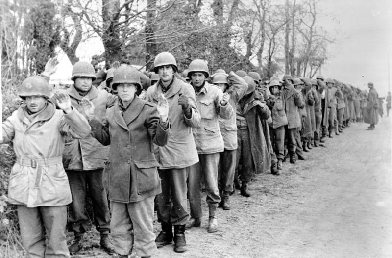
U.S. Army prisoners of war captured by German forces during the Battle of the Bulge in 1944. [Wikipedia]
One of the least studied aspects of combat is battle termination. Why do units in combat stop attacking or defending? Shifts in combat posture (attack, defend, delay, withdrawal) are usually voluntary, directed by a commander, but they can also be involuntary, as a result of direct or indirect enemy action. Why do involuntary changes in combat posture, known as breakpoints, occur?
As Chris pointed out in a previous post, the topic of breakpoints has only been addressed by two known studies since 1954. Most existing military combat models and wargames address breakpoints in at least a cursory way, usually through some calculation based on personnel casualties. Both of the breakpoints studies suggest that involuntary changes in posture are seldom related to casualties alone, however.
Current U.S. Army doctrine addresses changes in combat posture through discussions of culmination points in the attack, and transitions from attack to defense, defense to counterattack, and defense to retrograde. But these all pertain to voluntary changes, not breakpoints.
Army doctrinal literature has little to say about breakpoints, either in the context of friendly forces or potential enemy combatants. The little it does say relates to the effects of fire on enemy forces and is based on personnel and material attrition.
According to ADRP 1-02 Terms and Military Symbols, an enemy combat unit is considered suppressed after suffering 3% personnel casualties or material losses, neutralized by 10% losses, and destroyed upon sustaining 30% losses. The sources and methodology for deriving these figures is unknown, although these specific terms and numbers have been a part of Army doctrine for decades.
The joint U.S. Army and U.S. Marine Corps vision of future land combat foresees battlefields that are highly lethal and demanding on human endurance. How will such a future operational environment affect combat performance? Past experience undoubtedly offers useful insights but there seems to be little interest in seeking out such knowledge.
This week’s list of links is an odds-and-ends assortment.
David Vergun has an interview with General Stephen J. Townshend, commander of the U.S. Army Training and Doctrine Command (TRADOC) on the Army website about the need for smaller, lighter, and faster equipment for future warfare.
And finally, MeritTalk, a site focused on U.S. government information technology, has posted a piece, “Pentagon Wants An Early Warning System For Hybrid Warfare,” looking at the Defense Advanced Research Projects Agency’s (DARPA) ambitious Collection and Monitoring via Planning for Active Situational Scenarios (COMPASS) program, which will incorporate AI, game theory, modeling, and estimation technologies to attempt to decipher the often subtle signs that precede a full-scale attack.
In 1931, Lieutenant Colonel (later Brigadier General) Love, then a Medical Corps physician in the U.S. Army Medical Field Services School, published a study of American casualty data in the recent Great War, titled “War Casualties.”[1] This study was likely the source for tables used for casualty estimation by the U.S. Army through 1944.[2]
Love’s research was likely the basis for rate tables for calculating casualties that first appeared in the 1932 edition of the War Department’s Staff Officer’s Field Manual.[3]
Battle Casualties, including Killed, in Percent of Unit Strength, Staff Officer’s Field Manual (1932).
The 1932 Staff Officer’s Field Manual estimation methodology reflected Love’s sophisticated understanding of the factors influencing combat casualty rates. It showed that both the resistance and combat strength (and all of the factors that comprised it) of the enemy, as well as the equipment and state of training and discipline of the friendly troops had to be taken into consideration. The text accompanying the tables pointed out that loss rates in small units could be quite high and variable over time, and that larger formations took fewer casualties as a fraction of overall strength, and that their rates tended to become more constant over time. Casualties were not distributed evenly, but concentrated most heavily among the combat arms, and in the front-line infantry in particular. Attackers usually suffered higher loss rates than defenders. Other factors to be accounted for included the character of the terrain, the relative amount of artillery on each side, and the employment of gas.
The 1941 iteration of the Staff Officer’s Field Manual, now designated Field Manual (FM) 101-10[4], provided two methods for estimating battle casualties. It included the original 1932 Battle Casualties table, but the associated text no longer included the section outlining factors to be considered in calculating loss rates. This passage was moved to a note appended to a new table showing the distribution of casualties among the combat arms.
Rather confusingly, FM 101-10 (1941) presented a second table, Estimated Daily Losses in Campaign of Personnel, Dead and Evacuated, Per 1,000 of Actual Strength. It included rates for front line regiments and divisions, corps and army units, reserves, and attached cavalry. The rates were broken down by posture and tactical mission.
Estimated Daily Losses in Campaign of Personnel, Dead and Evacuated, Per 1,000 of Actual Strength, FM 101-10 (1941)
The source for this table is unknown, nor the method by which it was derived. No explanatory text accompanied it, but a footnote stated that “this table is intended primarily for use in school work and in field exercises.” The rates in it were weighted toward the upper range of the figures provided in the 1932 Battle Casualties table.
The October 1943 edition of FM 101-10 contained no significant changes from the 1941 version, except for the caveat that the 1932 Battle Casualties table “may or may not prove correct when applied to the present conflict.”
The October 1944 version of FM 101-10 incorporated data obtained from World War II experience.[5] While it also noted that the 1932 Battle Casualties table might not be applicable, the experiences of the U.S. II Corps in North Africa and one division in Italy were found to be in agreement with the table’s division and corps loss rates.
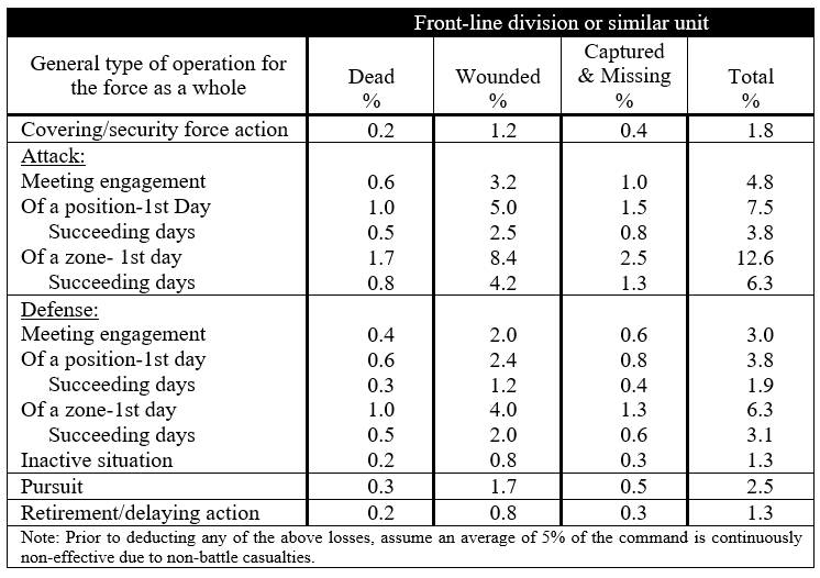
FM 101-10 (1944) included another new table, Estimate of Battle Losses for a Front-Line Division (in % of Actual Strength), meaning that it now provided three distinct methods for estimating battle casualties.
Estimate of Battle Losses for a Front-Line Division (in % of Actual Strength), FM 101-10 (1944)
Like the 1941 Estimated Daily Losses in Campaign table, the sources for this new table were not provided, and the text contained no guidance as to how or when it should be used. The rates it contained fell roughly within the span for daily rates for severe (6-8%) to maximum (12%) combat listed in the 1932 Battle Casualty table, but would produce vastly higher overall rates if applied consistently, much higher than the 1932 table’s 1% daily average.
FM 101-10 (1944) included a table showing the distribution of losses by branch for the theater based on experience to that date, except for combat in the Philippine Islands. The new chart was used in conjunction with the 1944 Estimate of Battle Losses for a Front-Line Division table to determine daily casualty distribution.
Distribution of Battle Losses–Theater of Operations, FM 101-10 (1944)
The final World War II version of FM 101-10 issued in August 1945[6] contained no new casualty rate tables, nor any revisions to the existing figures. It did finally effectively invalidate the 1932 Battle Casualties table by noting that “the following table has been developed from American experience in active operations and, of course, may not be applicable to a particular situation.” (original emphasis)
NOTES
[1] Albert G. Love, War Casualties, The Army Medical Bulletin, No. 24, (Carlisle Barracks, PA: 1931)
[2] This post is adapted from TDI, Casualty Estimation Methodologies Study, Interim Report (May 2005) (Altarum) (pp. 314-317).
[3] U.S. War Department, Staff Officer’s Field Manual, Part Two: Technical and Logistical Data (Government Printing Office, Washington, D.C., 1932)
[4] U.S. War Department, FM 101-10, Staff Officer’s Field Manual: Organization, Technical and Logistical Data (Washington, D.C., June 15, 1941)
[5] U.S. War Department, FM 101-10, Staff Officer’s Field Manual: Organization, Technical and Logistical Data (Washington, D.C., October 12, 1944)
[6] U.S. War Department, FM 101-10 Staff Officer’s Field Manual: Organization, Technical and Logistical Data (Washington, D.C., August 1, 1945)
Technology and the Human Factor in War by Trevor N. Dupuy
The Debate
It has become evident to many military theorists that technology has become increasingly important in war. In fact (even though many soldiers would not like to admit it) most such theorists believe that technology has actually reduced the significance of the human factor in war, In other words, the more advanced our military technology, these “technocrats” believe, the less we need to worry about the professional capability and competence of generals, admirals, soldiers, sailors, and airmen.
The technocrats believe that the results of the Kuwait, or Gulf, War of 1991 have confirmed their conviction. They cite the contribution to those results of the U.N. (mainly U.S.) command of the air, stealth aircraft, sophisticated guided missiles, and general electronic superiority, They believe that it was technology which simply made irrelevant the recent combat experience of the Iraqis in their long war with Iran.
Yet there are a few humanist military theorists who believe that the technocrats have totally misread the lessons of this century‘s wars! They agree that, while technology was important in the overwhelming U.N. victory, the principal reason for the tremendous margin of U.N. superiority was the better training, skill, and dedication of U.N. forces (again, mainly U.S.).
And so the debate rests. Both sides believe that the result of the Kuwait War favors their point of view, Nevertheless, an objective assessment of the literature in professional military journals, of doctrinal trends in the U.S. services, and (above all) of trends in the U.S. defense budget, suggest that the technocrats have stronger arguments than the humanists—or at least have been more convincing in presenting their arguments.
I suggest, however, that a completely impartial comparison of the Kuwait War results with those of other recent wars, and with some of the phenomena of World War II, shows that the humanists should not yet concede the debate.
I am a humanist, who is also convinced that technology is as important today in war as it ever was (and it has always been important), and that any national or military leader who neglects military technology does so to his peril and that of his country, But, paradoxically, perhaps to an extent even greater than ever before, the quality of military men is what wins wars and preserves nations.
To elevate the debate beyond generalities, and demonstrate convincingly that the human factor is at least as important as technology in war, I shall review eight instances in this past century when a military force has been successful because of the quality if its people, even though the other side was at least equal or superior in the technological sophistication of its weapons. The examples I shall use are:
Germany vs. the USSR in World War II
Germany vs. the West in World War II
Israel vs. Arabs in 1948, 1956, 1967, 1973 and 1982
The Vietnam War, 1965-1973
Britain vs. Argentina in the Falklands 1982
South Africans vs. Angolans and Cubans, 1987-88
The U.S. vs. Iraq, 1991
The demonstration will be based upon a marshaling of historical facts, then analyzing those facts by means of a little simple arithmetic.
Relative Combat Effectiveness Value (CEV)
The purpose of the arithmetic is to calculate relative combat effectiveness values (CEVs) of two opposing military forces. Let me digress to set up the arithmetic. Although some people who hail from south of the Mason-Dixon Line may be reluctant to accept the fact, statistics prove that the fighting quality of Northern soldiers and Southern soldiers was virtually equal in the American Civil War. (I invite those who might disagree to look at Livermore’s Numbers and Losses in the Civil War). That assumption of equality of the opposing troop quality in the Civil War enables me to assert that the successful side in every important battle in the Civil War was successful either because of numerical superiority or superior generalship. Three of Lee’s battles make the point:
Despite being outnumbered, Lee won at Antietam. (Though Antietam is sometimes claimed as a Union victory, Lee, the defender, held the battlefield; McClellan, the attacker, was repulsed.) The main reason for Lee’s success was that on a scale of leadership his generalship was worth 10, while McClellan was barely a 6.
Despite being outnumbered, Lee won at Chancellorsville because he was a 10 to Hooker’s 5.
Lee lost at Gettysburg mainly because he was outnumbered. Also relevant: Meade did not lose his nerve (like McClellan and Hooker) with generalship worth 8 to match Lee’s 8.
Let me use Antietam to show the arithmetic involved in those simple analyses of a rather complex subject:
The numerical strength of McClellan’s army was 89,000; Lee’s army was only 39,000 strong, but had the multiplier benefit of defensive posture. This enables us to calculate the theoretical combat power ratio of the Union Army to the Confederate Army as 1.4:1.0. In other words, with substantial preponderance of force, the Union Army should have been successful. (The combat power ratio of Confederates to Northerners, of course, was the reciprocal, or 0.71:1.04)
However, Lee held the battlefield, and a calculation of the actual combat power ratio of the two sides (based on accomplishment of mission, gaining or holding ground, and casualties) was a scant, but clear cut: 1.16:1.0 in favor of the Confederates. A ratio of the actual combat power ratio of the Confederate/Union armies (1.16) to their theoretical combat power (0.71) gives us a value of 1.63. This is the relative combat effectiveness of the Lee’s army to McClellan’s army on that bloody day. But, if we agree that the quality of the troops was the same, then the differential must essentially be in the quality of the opposing generals. Thus, Lee was a 10 to McClellan‘s 6.
The simple arithmetic equation[1] on which the above analysis was based is as follows:
CEV = (R/R)/(P/P)
When:
CEV is relative Combat Effectiveness Value
R/R is the actual combat power ratio
P/P is the theoretical combat power ratio.
At Antietam the equation was: 1.63 = 1.16/0.71.
We’ll be revisiting that equation in connection with each of our examples of the relative importance of technology and human factors.
Air Power and Technology
However, one more digression is required before we look at the examples. Air power was important in all eight of the 20th Century examples listed above. Offhand it would seem that the exercise of air superiority by one side or the other is a manifestation of technological superiority. Nevertheless, there are a few examples of an air force gaining air superiority with equivalent, or even inferior aircraft (in quality or numbers) because of the skill of the pilots.
However, the instances of such a phenomenon are rare. It can be safely asserted that, in the examples used in the following comparisons, the ability to exercise air superiority was essentially a technological superiority (even though in some instances it was magnified by human quality superiority). The one possible exception might be the Eastern Front in World War II, where a slight German technological superiority in the air was offset by larger numbers of Soviet aircraft, thanks in large part to Lend-Lease assistance from the United States and Great Britain.
The Battle of Kursk, 5-18 July, 1943
Following the surrender of the German Sixth Army at Stalingrad, on 2 February, 1943, the Soviets mounted a major winter offensive in south-central Russia and Ukraine which reconquered large areas which the Germans had overrun in 1941 and 1942. A brilliant counteroffensive by German Marshal Erich von Manstein‘s Army Group South halted the Soviet advance, and recaptured the city of Kharkov in mid-March. The end of these operations left the Soviets holding a huge bulge, or salient, jutting westward around the Russian city of Kursk, northwest of Kharkov.
The Germans promptly prepared a new offensive to cut off the Kursk salient, The Soviets energetically built field fortifications to defend the salient against expected German attacks. The German plan was for simultaneous offensives against the northern and southern shoulders of the base of the Kursk salient, Field Marshal Gunther von K1uge’s Army Group Center, would drive south from the vicinity of Orel, while Manstein’s Army Group South pushed north from the Kharkov area, The offensive was originally scheduled for early May, but postponements by Hitler, to equip his forces with new tanks, delayed the operation for two months, The Soviets took advantage of the delays to further improve their already formidable defenses.
The German attacks finally began on 5 July. In the north General Walter Model’s German Ninth Army was soon halted by Marshal Konstantin Rokossovski’s Army Group Center. In the south, however, German General Hermann Hoth’s Fourth Panzer Army and a provisional army commanded by General Werner Kempf, were more successful against the Voronezh Army Group of General Nikolai Vatutin. For more than a week the XLVIII Panzer Corps advanced steadily toward Oboyan and Kursk through the most heavily fortified region since the Western Front of 1918. While the Germans suffered severe casualties, they inflicted horrible losses on the defending Soviets. Advancing similarly further east, the II SS Panzer Corps, in the largest tank battle in history, repulsed a vigorous Soviet armored counterattack at Prokhorovka on July 12-13, but was unable to continue to advance.
The principal reason for the German halt was the fact that the Soviets had thrown into the battle General Ivan Konev’s Steppe Army Group, which had been in reserve. The exhausted, heavily outnumbered Germans had no comparable reserves to commit to reinvigorate their offensive.
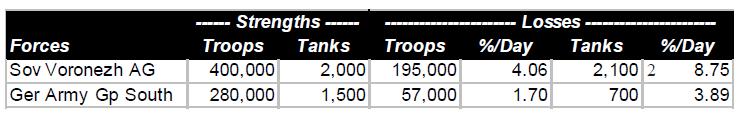
A comparison of forces and losses of the Soviet Voronezh Army Group and German Army Group South on the south face of the Kursk Salient is shown below. The strengths are averages over the 12 days of the battle, taking into consideration initial strengths, losses, and reinforcements.
A comparison of the casualty tradeoff can be found by dividing Soviet casualties by German strength, and German losses by Soviet strength. On that basis, 100 Germans inflicted 5.8 casualties per day on the Soviets, while 100 Soviets inflicted 1.2 casualties per day on the Germans, a tradeoff of 4.9 to 1.0
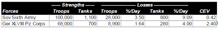
The statistics for the 8-day offensive of the German XLVIII Panzer Corps toward Oboyan are shown below. Also shown is the relative combat effectiveness value (CEV) of Germans and Soviets, as calculated by the TNDM. As was the case for the Battle of Antietam, this is derived from a mathematical comparison of the theoretical combat power ratio of the two forces (simply considering numbers and weapons characteristics), and the actual combat power ratios reflected by the battle results:
The calculated CEVs suggest that 100 German troops were the combat equivalent of 240 Soviet troops, comparably equipped. The casualty tradeoff in this battle shows that 100 Germans inflicted 5.15 casualties per day on the Soviets, while 100 Soviets inflicted 1.11 casualties per day on the Germans, a tradeoff of4.64. It is a rule of thumb that the casualty tradeoff is usually about the square of the CEV.
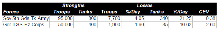
A similar comparison can be made of the two-day battle of Prokhorovka. Soviet accounts of that battle have claimed this as a great victory by the Soviet Fifth Guards Tank Army over the German II SS Panzer Corps. In fact, since the German advance was halted, the outcome was close to a draw, but with the advantage clearly in favor of the Germans.
The casualty tradeoff shows that 100 Germans inflicted 7.7 casualties per on the Soviets, while 100 Soviets inflicted 1.0 casualties per day on the Germans, for a tradeoff value of 7.7.
When the German offensive began, they had a slight degree of local air superiority. This was soon reversed by German and Soviet shifts of air elements, and during most of the offensive, the Soviets had a slender margin of air superiority. In terms of technology, the Germans probably had a slight overall advantage. However, the Soviets had more tanks and, furthermore, their T-34 was superior to any tank the Germans had available at the time. The CEV calculations demonstrate that the Germans had a great qualitative superiority over the Russians, despite near-equality in technology, and despite Soviet air superiority. The Germans lost the battle, but only because they were overwhelmed by Soviet numbers.
German Performance, Western Europe, 1943-1945
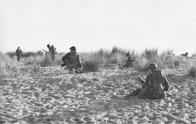
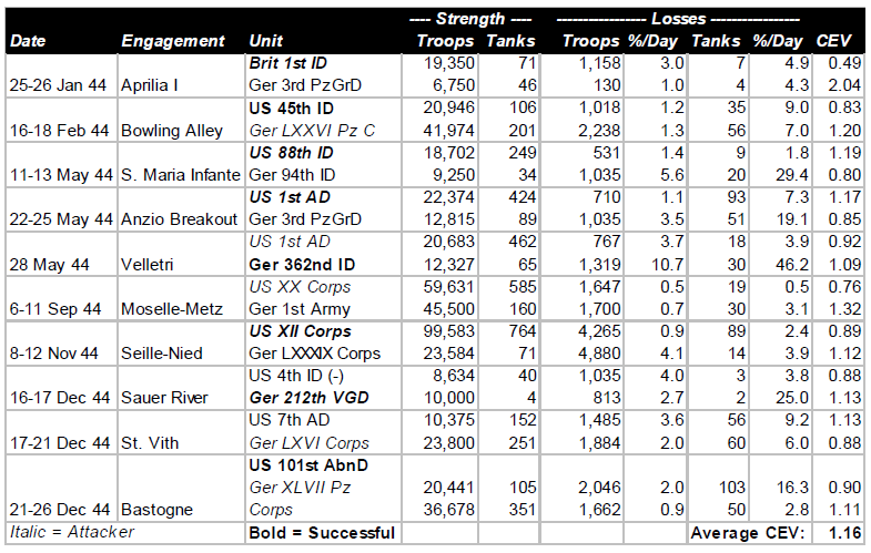
Beginning with operations between Salerno and Naples in September, 1943, through engagements in the closing days of the Battle of the Bulge in January, 1945, the pattern of German performance against the Western Allies was consistent. Some German units were better than others, and a few Allied units were as good as the best of the Germans. But on the average, German performance, as measured by CEV and casualty tradeoff, was better than the Western allies by a CEV factor averaging about 1.2, and a casualty tradeoff factor averaging about 1.5. Listed below are ten engagements from Italy and Northwest Europe during that 1944.
Technologically, German forces and those of the Western Allies were comparable. The Germans had a higher proportion of armored combat vehicles, and their best tanks were considerably better than the best American and British tanks, but the advantages were at least offset by the greater quantity of Allied armor, and greater sophistication of much of the Allied equipment. The Allies were increasingly able to achieve and maintain air superiority during this period of slightly less than two years.
The combination of vast superiority in numbers of troops and equipment, and in increasing Allied air superiority, enabled the Allies to fight their way slowly up the Italian boot, and between June and December, 1944, to drive from the Normandy beaches to the frontier of Germany. Yet the presence or absence of Allied air support made little difference in terms of either CEVs or casualty tradeoff values. Despite the defeats inflicted on them by the numerically superior Allies during the latter part of 1944, in December the Germans were able to mount a major offensive that nearly destroyed an American army corps, and threatened to drive at least a portion of the Allied armies into the sea.
Clearly, in their battles against the Soviets and the Western Allies, the Germans demonstrated that quality of combat troops was able consistently to overcome Allied technological and air superiority. It was Allied numbers, not technology, that defeated the quantitatively superior Germans.
The Six-Day War, 1967
The remarkable Israeli victories over far more numerous Arab opponents—Egyptian, Jordanian, and Syrian—in June, 1967 revealed an Israeli combat superiority that had not been suspected in the United States, the Soviet Union or Western Europe. This superiority was equally awesome on the ground as in the air. (By beginning the war with a surprise attack which almost wiped out the Egyptian Air Force, the Israelis avoided a serious contest with the one Arab air force large enough, and possibly effective enough, to challenge them.) The results of the three brief campaigns are summarized in the table below:
It should be noted that some Israelis who fought against the Egyptians and Jordanians also fought against the Syrians. Thus, the overall Arab numerical superiority was greater than would be suggested by adding the above strength figures, and was approximately 328,000 to 200,000.
It should also be noted that the technological sophistication of the Israeli and Arab ground forces was comparable. The only significant technological advantage of the Israelis was their unchallenged command of the air. (In terms of battle outcomes, it was irrelevant how they had achieved air superiority.) In fact this was a very significant advantage, the full import of which would not be realized until the next Arab-Israeli war.
The results of the Six Day War do not provide an unequivocal basis for determining the relative importance of human factors and technological superiority (as evidenced in the air). Clearly a major factor in the Israeli victories was the superior performance of their ground forces due mainly to human factors. At least as important in those victories was Israeli command of the air, in which both technology and human factors both played a part.
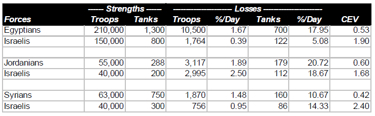
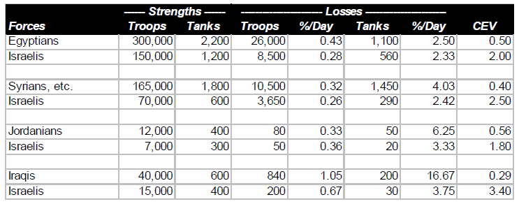
The October War, 1973
A better basis for comparing the relative importance of human factors and technology is provided by the results of the October War of 1973 (known to Arabs as the War of Ramadan, and to Israelis as the Yom Kippur War). In this war the Israeli unquestioned superiority in the air was largely offset by the Arabs possession of highly sophisticated Soviet air defense weapons.
One important lesson of this war was a reassessment of Israeli contempt for the fighting quality of Arab ground forces (which had stemmed from the ease with which they had won their ground victories in 1967). When Arab ground troops were protected from Israeli air superiority by their air defense weapons, they fought well and bravely, demonstrating that Israeli control of the air had been even more significant in 1967 than anyone had then recognized.
It should be noted that the total Arab (and Israeli) forces are those shown in the first two comparisons, above. A Jordanian brigade and two Iraqi divisions formed relatively minor elements of the forces under Syrian command (although their presence on the ground was significant in enabling the Syrians to maintain a defensive line when the Israelis threatened a breakthrough around 20 October). For the comparison of Jordanians and Iraqis the total strength is the total of the forces in the battles (two each) on which these comparisons are based.
One other thing to note is how the Israelis, possibly unconsciously, confirmed that validity of their CEVs with respect to Egyptians and Syrians by the numerical strengths of their deployments to the two fronts. Since the war ended up in a virtual stalemate on both fronts, the overall strength figures suggest rough equivalence of combat capability.
The CEV values shown in the above table are very significant in relation to the debate about human factors and technology, There was little if anything to choose between the technological sophistication of the two sides. The Arabs had more tanks than the Israelis, but (as Israeli General Avraham Adan once told the author) there was little difference in the quality of the tanks. The Israelis again had command of the air, but this was neutralized immediately over the battlefields by the Soviet air defense equipment effectively manned by the Arabs. Thus, while technology was of the utmost importance to both sides, enabling each side to prevent the enemy from gaining a significant advantage, the true determinant of battlefield outcomes was the fighting quality of the troops, And, while the Arabs fought bravely, the Israelis fought much more effectively. Human factors made the difference.
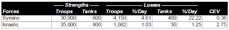
Israeli Invasion of Lebanon, 1982
In terms of the debate about the relative importance of human factors and technology, there are two significant aspects to this small war, in which Syrians forces and PLO guerrillas were the Arab participants. In the first place, the Israelis showed that their air technology was superior to the Syrian air defense technology, As a result, they regained complete control of the skies over the battlefields. Secondly, it provides an opportunity to include a highly relevant quotation.
The statistical comparison shows the results of the two major battles fought between Syrians and Israelis:
In assessing the above statistics, a quotation from the Israeli Chief of Staff, General Rafael Eytan, is relevant.
In late 1982 a group of retired American generals visited Israel and the battlefields in Lebanon. Just before they left for home, they had a meeting with General Eytan. One of the American generals asked Eytan the following question: “Since the Syrians were equipped with Soviet weapons, and your troops were equipped with American (or American-type) weapons, isn’t the overwhelming Israeli victory an indication of the superiority of American weapons technology over Soviet weapons technology?”
Eytan’s reply was classic: “If we had had their weapons, and they had had ours, the result would have been absolutely the same.”
One need not question how the Israeli Chief of Staff assessed the relative importance of the technology and human factors.
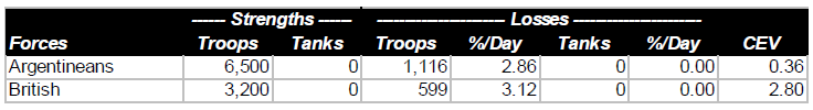
Falkland Islands War, 1982
It is difficult to get reliable data on the Falkland Islands War of 1982. Furthermore, the author of this article had not undertaken the kind of detailed analysis of such data as is available. However, it is evident from the information that is available about that war that its results were consistent with those of the other examples examined in this article.
The total strength of Argentine forces in the Falklands at the time of the British counter-invasion was slightly more than 13,000. The British appear to have landed close to 6,400 troops, although it may have been fewer. In any event, it is evident that not more than 50% of the total forces available to both sides were actually committed to battle. The Argentine surrender came 27 days after the British landings, but there were probably no more than six days of actual combat. During these battles the British performed admirably, the Argentinians performed miserably. (Save for their Air Force, which seems to have fought with considerable gallantry and effectiveness, at the extreme limit of its range.) The British CEV in ground combat was probably between 2.5 and 4.0. The statistics were at least close to those presented below:
It is evident from published sources that the British had no technological advantage over the Argentinians; thus the one-sided results of the ground battles were due entirely to British skill (derived from training and doctrine) and determination.
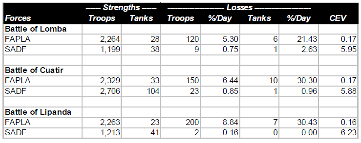
South African Operations in Angola, 1987-1988
Neither the political reasons for, nor political results of, the South African military interventions in Angola in the 1970s, and again in the late 1980s, need concern us in our consideration of the relative significance of technology and of human factors. The combat results of those interventions, particularly in 1987-1988 are, however, very relevant.
The operations between elements of the South African Defense Force (SADF) and forces of the Popular Movement for the Liberation of Angola (FAPLA) took place in southeast Angola, generally in the region east of the city of Cuito-Cuanavale. Operating with the SADF units were a few small units of Jonas Savimbi’s National Union for the Total Independence of Angola (UNITA). To provide air support to the SADF and UNITA ground forces, it would have been necessary for the South Africans to establish air bases either in Botswana, Southwest Africa (Namibia), or in Angola itself. For reasons that were largely political, they decided not to do that, and thus operated under conditions of FAPLA air supremacy. This led them, despite terrain generally unsuited for armored warfare, to use a high proportion of armored vehicles (mostly light armored cars) to provide their ground troops with some protection from air attack.
Summarized below are the results of three battles east of Cuito-Cuanavale in late 1987 and early 1988. Included with FAPLA forces are a few Cubans (mostly in armored units); included with the SADF forces are a few UNITA units (all infantry).
FAPLA had complete command of air, and substantial numbers of MiG-21 and MiG-23 sorties were flown against the South Africans in all of these battles. This technological superiority was probably partly offset by greater South African EW (electronic warfare) capability. The ability of the South Africans to operate effectively despite hostile air superiority was reminiscent of that of the Germans in World War II. It was a further demonstration that, no matter how important technology may be, the fighting quality of the troops is even more important.
The tank figures include armored cars. In the first of the three battles considered, FAPLA had by far the more powerful and more numerous medium tanks (20 to 0). In the other two, SADF had a slight or significant advantage in medium tank numbers and quality. But it didn’t seem to make much difference in the outcomes.
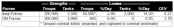
Kuwait War, 1991
The previous seven examples permit us to examine the results of Kuwait (or Second Gulf) War with more objectivity than might otherwise have possible. First, let’s look at the statistics. Note that the comparison shown below is for four days of ground combat, February 24-28, and shows only operations of U.S. forces against the Iraqis.
There can be no question that the single most important contribution to the overwhelming victory of U.S. and other U.N. forces was the air war that preceded, and accompanied, the ground operations. But two comments are in order. The air war alone could not have forced the Iraqis to surrender. On the other hand, it is evident that, even without the air war, U.S. forces would have readily overwhelmed the Iraqis, probably in more than four days, and with more than 285 casualties. But the outcome would have been hardly less one-sided.
The Vietnam War, 1965-1973
It is impossible to make the kind of mathematical analysis for the Vietnam War as has been done in the examples considered above. The reason is that we don’t have any good data on the Vietcong—North Vietnamese forces,
However, such quantitative analysis really isn’t necessary There can be no doubt that one of the opponents was a superpower, the most technologically advanced nation on earth, while the other side was what Lyndon Johnson called a “raggedy-ass little nation,” a typical representative of “the third world.“
Furthermore, even if we were able to make the analyses, they would very possibly be misinterpreted. It can be argued (possibly with some exaggeration) that the Americans won all of the battles. The detailed engagement analyses could only confirm this fact. Yet it is unquestionable that the United States, despite airpower and all other manifestations of technological superiority, lost the war. The human factor—as represented by the quality of American political (and to a lesser extent military) leadership on the one side, and the determination of the North Vietnamese on the other side—was responsible for this defeat.
Conclusion
In a recent article in the Armed Forces Journal International Col. Philip S. Neilinger, USAF, wrote: “Military operations are extremely difficult, if not impossible, for the side that doesn’t control the sky.” From what we have seen, this is only partly true. And while there can be no question that operations will always be difficult to some extent for the side that doesn’t control the sky, the degree of difficulty depends to a great degree upon the training and determination of the troops.
What we have seen above also enables us to view with a better perspective Colonel Neilinger’s subsequent quote from British Field Marshal Montgomery: “If we lose the war in the air, we lose the war and we lose it quickly.” That statement was true for Montgomery, and for the Allied troops in World War II. But it was emphatically not true for the Germans.
The examples we have seen from relatively recent wars, therefore, enable us to establish priorities on assuring readiness for war. It is without question important for us to equip our troops with weapons and other materiel which can match, or come close to matching, the technological quality of the opposition’s materiel. We must realize that we cannot—as some people seem to think—buy good forces, by technology alone. Even more important is to assure the fighting quality of the troops. That must be, by far, our first priority in peacetime budgets and in peacetime military activities of all sorts.
NOTES
[1] This calculation is automatic in analyses of historical battles by the Tactical Numerical Deterministic Model (TNDM).
[2] The initial tank strength of the Voronezh Army Group was about 1,100 tanks. About 3,000 additional Soviet tanks joined the battle between 6 and 12 July. At the end of the battle there were about 1,800 Soviet tanks operational in the battle area; at the same time there were about 1,000 German tanks still operational.
[3] The relative combat effectiveness value of each force is calculated in comparison to 1.0. Thus the CEV of the Germans is 2.40:1.0, while that of the Soviets is 0.42: 1.0. The opposing CEVs are always the reciprocals of each other.
Last autumn, U.S. Army Chief of Staff General Mark Milley asserted that “we are on the cusp of a fundamental change in the character of warfare, and specifically ground warfare. It will be highly lethal, very highly lethal, unlike anything our Army has experienced, at least since World War II.” He made these comments while describing the Army’s evolving Multi-Domain Battle concept for waging future combat against peer or near-peer adversaries.
It is possible that ground combat attrition in the future between peer or near-peer combatants may be comparable to the U.S. experience in World War II (although there were considerable differences between the experiences of the various belligerents). Combat losses could be heavier. It certainly seems likely that they would be higher than those experienced by U.S. forces in recent counterinsurgency operations.
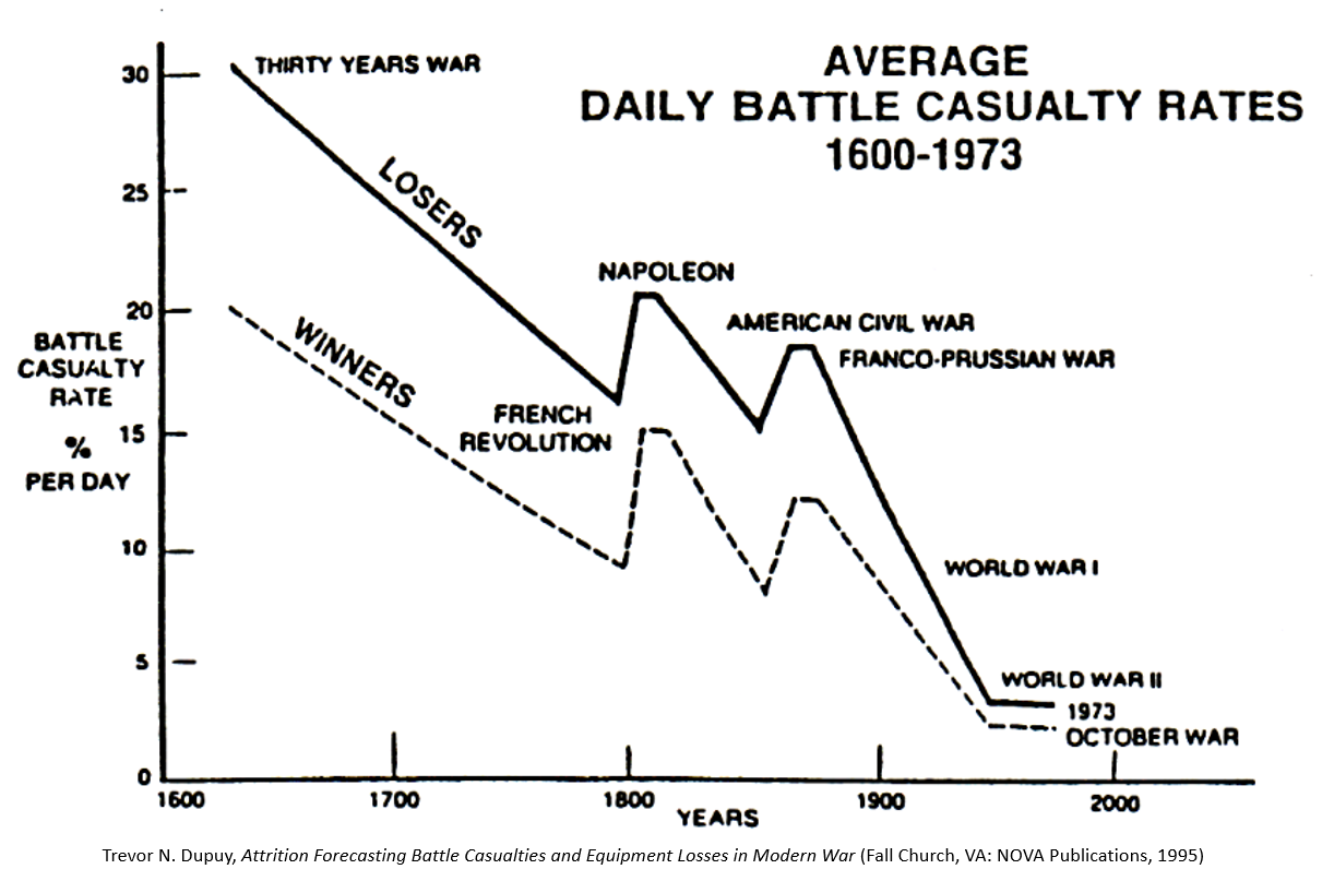
Dupuy documented a clear relationship over time between increasing weapon lethality, greater battlefield dispersion, and declining casualty rates in conventional combat. Even as weapons became more lethal, greater dispersal in frontage and depth among ground forces led daily personnel loss rates in battle to decrease.
The average daily battle casualty rate in combat has been declining since 1600 as a consequence. Since battlefield weapons continue to increase in lethality and troops continue to disperse in response, it seems logical to presume the trend in loss rates continues to decline, although this may not necessarily be the case. There were two instances in the 19th century where daily battle casualty rates increased—during the Napoleonic Wars and the American Civil War—before declining again. Dupuy noted that combat casualty rates in the 1973 Arab-Israeli War remained roughly the same as those in World War II (1939-45), almost thirty years earlier. Further research is needed to determine if average daily personnel loss rates have indeed continued to decrease into the 21st century.
Dupuy also discovered that, as with battle outcomes, casualty rates are influenced by the circumstantial variables of combat. Posture, weather, terrain, season, time of day, surprise, fatigue, level of fortification, and “all out” efforts affect loss rates. (The combat loss rates of armored vehicles, artillery, and other other weapons systems are directly related to personnel loss rates, and are affected by many of the same factors.) Consequently, yet counterintuitively, he could find no direct relationship between numerical force ratios and combat casualty rates. Combat power ratios which take into account the circumstances of combat do affect casualty rates; forces with greater combat power inflict higher rates of casualties than less powerful forces do.
Winning forces suffer lower rates of combat losses than losing forces do, whether attacking or defending. (It should be noted that there is a difference between combat loss rates and numbers of losses. Depending on the circumstances, Dupuy found that the numerical losses of the winning and losing forces may often be similar, even if the winner’s casualty rate is lower.)
Dupuy’s research confirmed the fact that the combat loss rates of smaller forces is higher than that of larger forces. This is in part due to the fact that smaller forces have a larger proportion of their troops exposed to enemy weapons; combat casualties tend to concentrated in the forward-deployed combat and combat support elements. Dupuy also surmised that Prussian military theorist Carl von Clausewitz’s concept of friction plays a role in this. The complexity of interactions between increasing numbers of troops and weapons simply diminishes the lethal effects of weapons systems on real world battlefields.
Somewhat unsurprisingly, higher quality forces (that better manage the ambient effects of friction in combat) inflict casualties at higher rates than those with less effectiveness. This can be seen clearly in the disparities in casualties between German and Soviet forces during World War II, Israeli and Arab combatants in 1973, and U.S. and coalition forces and the Iraqis in 1991 and 2003.
Combat Loss Rates on Future Battlefields
What do Dupuy’s combat attrition verities imply about casualties in future battles? As a baseline, he found that the average daily combat casualty rate in Western Europe during World War II for divisional-level engagements was 1-2% for winning forces and 2-3% for losing ones. For a divisional slice of 15,000 personnel, this meant daily combat losses of 150-450 troops, concentrated in the maneuver battalions (The ratio of wounded to killed in modern combat has been found to be consistently about 4:1. 20% are killed in action; the other 80% include mortally wounded/wounded in action, missing, and captured).
It seems reasonable to conclude that future battlefields will be less densely occupied. Brigades, battalions, and companies will be fighting in spaces formerly filled with armies, corps, and divisions. Fewer troops mean fewer overall casualties, but the daily casualty rates of individual smaller units may well exceed those of WWII divisions. Smaller forces experience significant variation in daily casualties, but Dupuy established average daily rates for them as shown below.
For example, based on Dupuy’s methodology, the average daily loss rate unmodified by combat variables for brigade combat teams would be 1.8% per day, battalions would be 8% per day, and companies 21% per day. For a brigade of 4,500, that would result in 81 battle casualties per day, a battalion of 800 would suffer 64 casualties, and a company of 120 would lose 27 troops. These rates would then be modified by the circumstances of each particular engagement.
Several factors could push daily casualty rates down. Milley envisions that U.S. units engaged in an anti-access/area denial environment will be constantly moving. A low density, highly mobile battlefield with fluid lines would be expected to reduce casualty rates for all sides. High mobility might also limit opportunities for infantry assaults and close quarters combat. The high operational tempo will be exhausting, according to Milley. This could also lower loss rates, as the casualty inflicting capabilities of combat units decline with each successive day in battle.
It is not immediately clear how cyberwarfare and information operations might influence casualty rates. One combat variable they might directly impact would be surprise. Dupuy identified surprise as one of the most potent combat power multipliers. A surprised force suffers a higher casualty rate and surprisers enjoy lower loss rates. Russian combat doctrine emphasizes using cyber and information operations to achieve it and forces with degraded situational awareness are highly susceptible to it. As Zelenopillya demonstrated, surprise attacks with modern weapons can be devastating.
Some factors could push combat loss rates up. Long-range precision weapons could expose greater numbers of troops to enemy fires, which would drive casualties up among combat support and combat service support elements. Casualty rates historically drop during night time hours, although modern night-vision technology and persistent drone reconnaissance might will likely enable continuous night and day battle, which could result in higher losses.
Drawing solid conclusions is difficult but the question of future battlefield attrition is far too important not to be studied with greater urgency. Current policy debates over whether or not the draft should be reinstated and the proper size and distribution of manpower in active and reserve components of the Army hinge on getting this right. The trend away from mass on the battlefield means that there may not be a large margin of error should future combat forces suffer higher combat casualties than expected.
Staff Sgt. Braxton Pernice, 6th Battalion, 1st Security Force Assistance Brigade, is pinned his Pathfinder Badge by a fellow 1st SFAB Soldier Nov. 3, 2017, at Fort Benning, Ga., following his graduation from Pathfinder School. Pernice is one of three 1st SFAB Soldiers to graduate the school since the formation of the 1st SFAB. He and Sgt 1st Class Rachel Lyons and Capt. Travis Lowe, all with 6th Bn., 1st SFAB, were among 42 students of Pathfinder School class 001-18 to earn their badge. (U.S. Army photo by Spc. Noelle E. Wiehe)
Many will also be watching to see if the SFAB concept validates the Army’s revamped approach to Security Force Assistance (SFA)—an umbrella term for whole-of-government support provided to develop the capability and capacity of foreign security forces and institutions. SFA has long been one of the U.S. government’s primary response to threats of insurgency and terrorism around the world, but its record of success is decidedly mixed.
Earlier this month, the 1st SFAB commander Colonel Scott Jackson reportedly briefed General Joseph Votel, who heads U.S. Central Command, that his unit had less than eight months of training and preparation, instead of an expected 12 months. His personnel had been rushed through the six-week Military Advisor Training Academy curriculum in only two weeks, and that the command suffered from personnel shortages. Votel reportedly passed these concerns to U.S. Army Chief of Staff General Mark Milley.
Competing Mission Priorities
Milley’s brainchild, the SFABs are intended to improve the Army’s ability to conduct SFA and to relieve line Brigade Combat Teams (BCTs) of responsibility for conducting it. Committing BCTs to SFA missions has been seen as both keeping them from more important conventional missions and inhibiting their readiness for high-intensity combat.
However, 1st SFAB may be caught out between two competing priorities: to adequately train Afghan forces and also to partner with and support them in combat operations. The SFABs are purposely optimized for training and advising, but they are not designed for conducting combat operations. They lack a BCT’s command, control and intelligence and combat assets. Some veteran military advisors have pointed out that BCTs are able to control battlespace and possess organic force protection, two capabilities the SFABs lack. While SFAB personnel will advise and accompany Afghan security forces in the field, they will not be able to support them in combat with them the way BCTs can. The Army will also have to deploy additional combat troops to provide sufficient force protection for 1st SFAB’s trainers.
Institutional Questions
The deviating requirements for training and combat advising may be the reason the Army appears to be providing the SFABs with capabilities that resemble those of Army Special Forces (ARSOF) personnel and units. ARSOF’s primary mission is to operate “by, with and through” indigenous forces. While Milley made clear in the past that the SFABs were not ARSOF, they do appear to include some deliberate similarities. While organized overall as a conventional BCT, the SFAB’s basic tactical teams include 12 personnel, like an ARSOF Operational Detachment A (ODA). Also like an ODA, the SFAB teams include intelligence and medical non-commissioned officers, and are also apparently being assigned dedicated personnel for calling in air and fire support (It is unclear from news reports if the SFAB teams include regular personnel trained in basic for call for fire techniques or if they are being given highly-skilled joint terminal attack controllers (JTACs).)
SFAB personnel have been selected using criteria used for ARSOF recruitment and Army Ranger physical fitness standards. They are being given foreign language training at the Military Advisor Training Academy at Fort Benning, Georgia.
The SFAB concept has drawn some skepticism from the ARSOF community, which sees the train, advise, and assist mission as belonging to it. There are concerns that SFABs will compete with ARSOF for qualified personnel and the Army has work to do to create a viable career path for dedicated military advisors. However, as Milley has explained, there are not nearly enough ARSOF personnel to effectively staff the Army’s SFA requirements, let alone meet the current demand for other ARSOF missions.
An Enduring Mission
Single-handedly rescuing a floundering 16-year, $70 billion effort to create an effective Afghan army as well as a national policy that suffers from basic strategic contradictions seems like a tall order for a brand-new, understaffed Army unit. At least one veteran military advisor has asserted that 1st SFAB is being “set up to fail.”
Yet, regardless of how well it performs, the SFA requirement will neither diminish nor go away. The basic logic behind the SFAB concept remains valid. It is possible that a problematic deployment could inhibit future recruiting, but it seems more likely that the SFABs and Army military advising will evolve as experience accumulates. SFA may or may not be a strategic “game changer” in Afghanistan, but as a former Army combat advisor stated, “It sounds low risk and not expensive, even when it is, [but] it’s not going away whether it succeeds or fails.”
The thinking of the services proceeds from a basic idea:
Victory in future combat will be determined by how successfully commanders can understand, visualize, and describe the battlefield to their subordinate commands, thus allowing for more rapid decisionmaking to exploit the initiative and create positions of relative advantage.
In order to create this common understanding, TRADOC and ACC are seeking to blend the conceptualization of their respective operating concepts.
The Army’s…operational framework is a cognitive tool used to assist commanders and staffs in clearly visualizing and describing the application of combat power in time, space, and purpose… The Army’s operational and battlefield framework is, by the reality and physics of the land domain, generally geographically focused and employed in multiple echelons.
The mission of the Air Force is to fly, fight, and win—in air, space, and cyberspace. With this in mind, and with the inherent flexibility provided by the range and speed of air, space, and cyber power, the ACC construct for visualizing and describing operations in time and space has developed differently from the Army’s… One key difference between the two constructs is that while the Army’s is based on physical location of friendly and enemy assets and systems, ACC’s is typically focused more on the functions conducted by friendly and enemy assets and systems. Focusing on the functions conducted by friendly and enemy forces allows coordinated employment and integration of air, space, and cyber effects in the battlespace to protect or exploit friendly functions while degrading or defeating enemy functions across geographic boundaries to create and exploit enemy vulnerabilities and achieve a continuing advantage.
Despite having “somewhat differing perspectives on mission command versus C2 and on a battlefield framework that is oriented on forces and geography versus one that is oriented on function and time,” it turns out that the services’ respective conceptualizations of their operating concepts are not incompatible. The first cut on an integrated concept yielded the diagram above. As Perkins and Holmes point out,
The only noncommon area between these two frameworks is the Air Force’s Adversary Strategic area. This area could easily be accommodated into the Army’s existing framework with the addition of Strategic Deep Fires—an area over the horizon beyond the range of land-based systems, thus requiring cross-domain fires from the sea, air, and space.
Perkins and Holmes go on to map out the next steps.
In the coming year, the Army and Air Force will be conducting a series of experiments and initiatives to help determine the essential components of MDB C2. Between the Services there is a common understanding of the future operational environment, the macro-level problems that must be addressed, and the capability gaps that currently exist. Potential solutions require us to ask questions differently, to ask different questions, and in many cases to change our definitions.
Their expectation is that “Frameworks will tend to merge—not as an either/or binary choice—but as a realization that effective cross-domain operations on the land and sea, in the air, as well as cyber and electromagnetic domains will require a merged framework and a common operating picture.”