Tag Trevor N. Dupuy

Scoring Weapons And Aggregation In Trevor Dupuy’s Combat Models

[The article below is reprinted from the October 1997 edition of The International TNDM Newsletter.]

Consistent Scoring of Weapons and Aggregation of Forces:
The Cornerstone of Dupuy’s Quantitative Analysis of Historical Land Battles
by
James G. Taylor, PhD,
Dept. of Operations Research, Naval Postgraduate School

Introduction

Col. Trevor N. Dupuy was an American original, especially as regards the quantitative study of warfare. As with many prophets, he was not entirely appreciated in his own land, particularly its Military Operations Research (OR) community. However, after becoming rather familiar with the details of his mathematical modeling of ground combat based on historical data, I became aware of the basic scientific soundness of his approach. Unfortunately, his documentation of methodology was not always accepted by others, many of whom appeared to confuse lack of mathematical sophistication in his documentation with lack of scientific validity of his basic methodology.

The purpose of this brief paper is to review the salient points of Dupuy’s methodology from a system’s perspective, i.e., to view his methodology as a system, functioning as an organic whole to capture the essence of past combat experience (with an eye towards extrapolation into the future). The advantage of this perspective is that it immediately leads one to the conclusion that if one wants to use some functional relationship derived from Dupuy’s work, then one should use his methodologies for scoring weapons, aggregating forces, and adjusting for operational circumstances; since this consistency is the only guarantee of being able to reproduce historical results and to project them into the future.

Implications (of this system’s perspective on Dupuy’s work) for current DOD models will be discussed. In particular, the Military OR community has developed quantitative methods for imputing values to weapon systems based on their attrition capability against opposing forces and force interactions.[1] One such approach is the so-called antipotential-potential method[2] used in TACWAR[3] to score weapons. However, one should not expect such scores to provide valid casualty estimates when combined with historically derived functional relationships such as the so-called ATLAS casualty-rate curves[4] used in TACWAR, because a different “yard-stick” (i.e. measuring system for estimating the relative combat potential of opposing forces) was used to develop such a curve.

Overview of Dupuy’s Approach

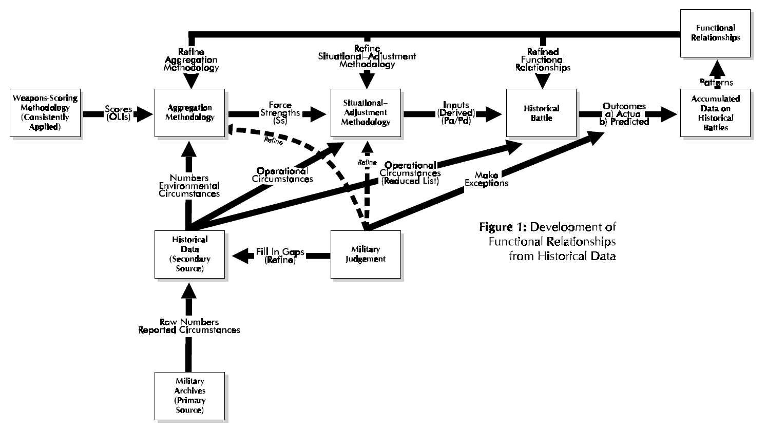
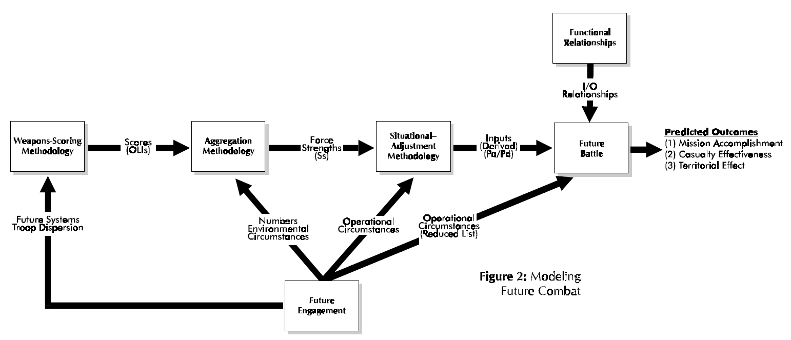
This section briefly outlines the salient features of Dupuy’s approach to the quantitative analysis and modeling of ground combat as embodied in his Tactical Numerical Deterministic Model (TNDM) and its predecessor the Quantified Judgment Model (QJM). The interested reader can find details in Dupuy [1979] (see also Dupuy [1985][5], [1987], [1990]). Here we will view Dupuy’s methodology from a system approach, which seeks to discern its various components and their interactions and to view these components as an organic whole. Essentially Dupuy’s approach involves the development of functional relationships from historical combat data (see Fig. 1) and then using these functional relationships to model future combat (see Fig, 2).

At the heart of Dupuy’s method is the investigation of historical battles and comparing the relationship of inputs (as quantified by relative combat power, denoted as Pa/Pd for that of the attacker relative to that of the defender in Fig. l)(e.g. see Dupuy [1979, pp. 59-64]) to outputs (as quantified by extent of mission accomplishment, casualty effectiveness, and territorial effectiveness; see Fig. 2) (e.g. see Dupuy [1979, pp. 47-50]), The salient point is that within this scheme, the main input[6] (i.e. relative combat power) to a historical battle is a derived quantity. It is computed from formulas that involve three essential aspects: (1) the scoring of weapons (e.g, see Dupuy [1979, Chapter 2 and also Appendix A]), (2) aggregation methodology for a force (e.g. see Dupuy [1979, pp. 43-46 and 202-203]), and (3) situational-adjustment methodology for determining the relative combat power of opposing forces (e.g. see Dupuy [1979, pp. 46-47 and 203-204]). In the force-aggregation step the effects on weapons of Dupuy’s environmental variables and one operational variable (air superiority) are considered[7], while in the situation-adjustment step the effects on forces of his behavioral variables[8] (aggregated into a single factor called the relative combat effectiveness value (CEV)) and also the other operational variables are considered (Dupuy [1987, pp. 86-89])

Figure 1.

Moreover, any functional relationships developed by Dupuy depend (unless shown otherwise) on his computational system for derived quantities, namely OLls, force strengths, and relative combat power. Thus, Dupuy’s results depend in an essential manner on his overall computational system described immediately above. Consequently, any such functional relationship (e.g. casualty-rate curve) directly or indirectly derivative from Dupuy‘s work should still use his computational methodology for determination of independent-variable values.

Fig l also reveals another important aspect of Dupuy’s work, the development of reliable data on historical battles, Military judgment plays an essential role in this development of such historical data for a variety of reasons. Dupuy was essentially the only source of new secondary historical data developed from primary sources (see McQuie [1970] for further details). These primary sources are well known to be both incomplete and inconsistent, so that military judgment must be used to fill in the many gaps and reconcile observed inconsistencies. Moreover, military judgment also generates the working hypotheses for model development (e.g. identification of significant variables).

At the heart of Dupuy’s quantitative investigation of historical battles and subsequent model development is his own weapons-scoring methodology, which slowly evolved out of study efforts by the Historical Evaluation Research Organization (HERO) and its successor organizations (cf. HERO [1967] and compare with Dupuy [1979]). Early HERO [1967, pp. 7-8] work revealed that what one would today call weapons scores developed by other organizations were so poorly documented that HERO had to create its own methodology for developing the relative lethality of weapons, which eventually evolved into Dupuy’s Operational Lethality Indices (OLIs). Dupuy realized that his method was arbitrary (as indeed is its counterpart, called the operational definition, in formal scientific work), but felt that this would be ameliorated if the weapons-scoring methodology be consistently applied to historical battles. Unfortunately, this point is not clearly stated in Dupuy’s formal writings, although it was clearly (and compellingly) made by him in numerous briefings that this author heard over the years.

Figure 2.

In other words, from a system’s perspective, the functional relationships developed by Colonel Dupuy are part of his analysis system that includes this weapons-scoring methodology consistently applied (see Fig. l again). The derived functional relationships do not stand alone (unless further empirical analysis shows them to hold for any weapons-scoring methodology), but function in concert with computational procedures. Another essential part of this system is Dupuy‘s aggregation methodology, which combines numbers, environmental circumstances, and weapons scores to compute the strength (S) of a military force. A key innovation by Colonel Dupuy [1979, pp. 202- 203] was to use a nonlinear (more precisely, a piecewise-linear) model for certain elements of force strength. This innovation precluded the occurrence of military absurdities such as air firepower being fully substitutable for ground firepower, antitank weapons being fully effective when armor targets are lacking, etc‘ The final part of this computational system is Dupuy’s situational-adjustment methodology, which combines the effects of operational circumstances with force strengths to determine relative combat power, e.g. Pa/Pd.

To recapitulate, the determination of an Operational Lethality Index (OLI) for a weapon involves the combination of weapon lethality, quantified in terms of a Theoretical Lethality Index (TLI) (e.g. see Dupuy [1987, p. 84]), and troop dispersion[9] (e.g. see Dupuy [1987, pp. 84- 85]). Weapons scores (i.e. the OLIs) are then combined with numbers (own side and enemy) and combat- environment factors to yield force strength. Six[10] different categories of weapons are aggregated, with nonlinear (i.e. piecewise-linear) models being used for the following three categories of weapons: antitank, air defense, and air firepower (i.e. c1ose—air support). Operational, e.g. mobility, posture, surprise, etc. (Dupuy [1987, p. 87]), and behavioral variables (quantified as a relative combat effectiveness value (CEV)) are then applied to force strength to determine a side’s combat-power potential.

Requirement for Consistent Scoring of Weapons, Force Aggregation, and Situational Adjustment for Operational Circumstances

The salient point to be gleaned from Fig.1 and 2 is that the same (or at least consistent) weapons—scoring, aggregation, and situational—adjustment methodologies be used for both developing functional relationships and then playing them to model future combat. The corresponding computational methods function as a system (organic whole) for determining relative combat power, e.g. Pa/Pd. For the development of functional relationships from historical data, a force ratio (relative combat power of the two opposing sides, e.g. attacker’s combat power divided by that of the defender, Pa/Pd is computed (i.e. it is a derived quantity) as the independent variable, with observed combat outcome being the dependent variable. Thus, as discussed above, this force ratio depends on the methodologies for scoring weapons, aggregating force strengths, and adjusting a force’s combat power for the operational circumstances of the engagement. It is a priori not clear that different scoring, aggregation, and situational-adjustment methodologies will lead to similar derived values. If such different computational procedures were to be used, these derived values should be recomputed and the corresponding functional relationships rederived and replotted.

However, users of the Tactical Numerical Deterministic Model (TNDM) (or for that matter, its predecessor, the Quantified Judgment Model (QJM)) need not worry about this point because it was apparently meticulously observed by Colonel Dupuy in all his work. However, portions of his work have found their way into a surprisingly large number of DOD models (usually not explicitly acknowledged), but the context and range of validity of historical results have been largely ignored by others. The need for recalibration of the historical data and corresponding functional relationships has not been considered in applying Dupuy’s results for some important current DOD models.

Implications for Current DOD Models

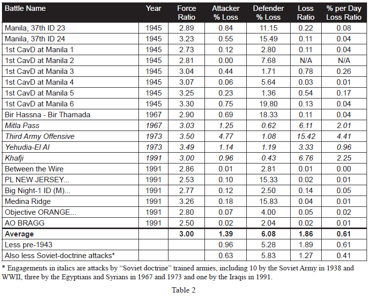
A number of important current DOD models (namely, TACWAR and JICM discussed below) make use of some of Dupuy’s historical results without recalibrating functional relationships such as loss rates and rates of advance as a function of some force ratio (e.g. Pa/Pd). As discussed above, it is not clear that such a procedure will capture the essence of past combat experience. Moreover, in calculating losses, Dupuy first determines personnel losses (expressed as a percent loss of personnel strength, i.e., number of combatants on a side) and then calculates equipment losses as a function of this casualty rate (e.g., see Dupuy [1971, pp. 219-223], also [1990, Chapters 5 through 7][11]). These latter functional relationships are apparently not observed in the models discussed below. In fact, only Dupuy (going back to Dupuy [1979][12] takes personnel losses to depend on a force ratio and other pertinent variables, with materiel losses being taken as derivative from this casualty rate.

For example, TACWAR determines personnel losses[13] by computing a force ratio and then consulting an appropriate casualty-rate curve (referred to as empirical data), much in the same fashion as ATLAS did[14]. However, such a force ratio is computed using a linear model with weapon values determined by the so-called antipotential-potential method[15]. Unfortunately, this procedure may not be consistent with how the empirical data (i.e. the casualty-rate curves) was developed. Further research is required to demonstrate that valid casualty estimates are obtained when different weapon scoring, aggregation, and situational-adjustment methodologies are used to develop casualty-rate curves from historical data and to use them to assess losses in aggregated combat models. Furthermore, TACWAR does not use Dupuy’s model for equipment losses (see above), although it does purport, as just noted above, to use “historical data” (e.g., see Kerlin et al. [1975, p. 22]) to compute personnel losses as a function (among other things) of a force ratio (given by a linear relationship), involving close air support values in a way never used by Dupuy. Although their force-ratio determination methodology does have logical and mathematical merit, it is not the way that the historical data was developed.

Moreover, RAND (Allen [1992]) has more recently developed what is called the situational force scoring (SFS) methodology for calculating force ratios in large-scale, aggregated-force combat situations to determine loss and movement rates. Here, SFS refers essentially to a force- aggregation and situation-adjustment methodology, which has many conceptual elements in common with Dupuy‘s methodology (except, most notably, extensive testing against historical data, especially documentation of such efforts). This SFS was originally developed for RSAS[16] and is today used in JICM[17]. It also apparently uses a weapon-scoring system developed at RAND[18]. It purports (no documentation given [citation of unpublished work]) to be consistent with historical data (including the ATLAS casualty-rate curves) (Allen [1992, p.41]), but again no consideration is given to recalibration of historical results for different weapon scoring, force-aggregation, and situational-adjustment methodologies. SFS emphasizes adjusting force strengths according to operational circumstances (the “situation”) of the engagement (including surprise), with many innovative ideas (but in some major ways has little connection with previous work of others[19]). The resulting model contains many more details than historical combat data would support. It also is methodology that differs in many essential ways from that used previously by any investigator. In particular, it is doubtful that it develops force ratios in a manner consistent with Dupuy’s work.

Final Comments

Use of (sophisticated) mathematics for modeling past historical combat (and extrapolating it into the future for planning purposes) is no reason for ignoring Dupuy’s work. One would think that the current Military OR community would try to understand Dupuy’s work before trying to improve and extend it. In particular, Colonel Dupuy’s various computational procedures (including constants) must be considered as an organic whole (i.e. a system) supporting the development of functional relationships. If one ignores this computational system and simply tries to use some isolated aspect, the result may be interesting and even logically sound, but it probably lacks any scientific validity.

REFERENCES

P. Allen, “Situational Force Scoring: Accounting for Combined Arms Effects in Aggregate Combat Models,” N-3423-NA, The RAND Corporation, Santa Monica, CA, 1992.

L. B. Anderson, “A Briefing on Anti-Potential Potential (The Eigen-value Method for Computing Weapon Values), WP-2, Project 23-31, Institute for Defense Analyses, Arlington, VA, March 1974.

B. W. Bennett, et al, “RSAS 4.6 Summary,” N-3534-NA, The RAND Corporation, Santa Monica, CA, 1992.

B. W. Bennett, A. M. Bullock, D. B. Fox, C. M. Jones, J. Schrader, R. Weissler, and B. A. Wilson, “JICM 1.0 Summary,” MR-383-NA, The RAND Corporation, Santa Monica, CA, 1994.

P. K. Davis and J. A. Winnefeld, “The RAND Strategic Assessment Center: An Overview and Interim Conclusions About Utility and Development Options,” R-2945-DNA, The RAND Corporation, Santa Monica, CA, March 1983.

T.N, Dupuy, Numbers. Predictions and War: Using History to Evaluate Combat Factors and Predict the Outcome of Battles, The Bobbs-Merrill Company, Indianapolis/New York, 1979,

T.N. Dupuy, Numbers Predictions and War, Revised Edition, HERO Books, Fairfax, VA 1985.

T.N. Dupuy, Understanding War: History and Theory of Combat, Paragon House Publishers, New York, 1987.

T.N. Dupuy, Attrition: Forecasting Battle Casualties and Equipment Losses in Modem War, HERO Books, Fairfax, VA, 1990.

General Research Corporation (GRC), “A Hierarchy of Combat Analysis Models,” McLean, VA, January 1973.

Historical Evaluation and Research Organization (HERO), “Average Casualty Rates for War Games, Based on Historical Data,” 3 Volumes in 1, Dunn Loring, VA, February 1967.

E. P. Kerlin and R. H. Cole, “ATLAS: A Tactical, Logistical, and Air Simulation: Documentation and User’s Guide,” RAC-TP-338, Research Analysis Corporation, McLean, VA, April 1969 (AD 850 355).

E.P. Kerlin, L.A. Schmidt, A.J. Rolfe, M.J. Hutzler, and D,L. Moody, “The IDA Tactical Warfare Model: A Theater-Level Model of Conventional, Nuclear, and Chemical Warfare, Volume II- Detailed Description” R-21 1, Institute for Defense Analyses, Arlington, VA, October 1975 (AD B009 692L).

R. McQuie, “Military History and Mathematical Analysis,” Military Review 50, No, 5, 8-17 (1970).

S.M. Robinson, “Shadow Prices for Measures of Effectiveness, I: Linear Model,” Operations Research 41, 518-535 (1993).

J.G. Taylor, Lanchester Models of Warfare. Vols, I & II. Operations Research Society of America, Alexandria, VA, 1983. (a)

J.G. Taylor, “A Lanchester-Type Aggregated-Force Model of Conventional Ground Combat,” Naval Research Logistics Quarterly 30, 237-260 (1983). (b)

NOTES

[1] For example, see Taylor [1983a, Section 7.18], which contains a number of examples. The basic references given there may be more accessible through Robinson [I993].

[2] This term was apparently coined by L.B. Anderson [I974] (see also Kerlin et al. [1975, Chapter I, Section D.3]).

[3] The Tactical Warfare (TACWAR) model is a theater-level, joint-warfare, computer-based combat model that is currently used for decision support by the Joint Staff and essentially all CINC staffs. It was originally developed by the Institute for Defense Analyses in the mid-1970s (see Kerlin et al. [1975]), originally referred to as TACNUC, which has been continually upgraded until (and including) the present day.

[4] For example, see Kerlin and Cole [1969], GRC [1973, Fig. 6-6], or Taylor [1983b, Fig. 5] (also Taylor [1983a, Section 7.13]).

[5] The only apparent difference between Dupuy [1979] and Dupuy [1985] is the addition of an appendix (Appendix C “Modified Quantified Judgment Analysis of the Bekaa Valley Battle”) to the end of the latter (pp. 241-251). Hence, the page content is apparently the same for these two books for pp. 1-239.

[6] Technically speaking, one also has the engagement type and possibly several other descriptors (denoted in Fig. 1 as reduced list of operational circumstances) as other inputs to a historical battle.

[7] In Dupuy [1979, e.g. pp. 43-46] only environmental variables are mentioned, although basically the same formulas underlie both Dupuy [1979] and Dupuy [1987]. For simplicity, Fig. 1 and 2 follow this usage and employ the term “environmental circumstances.”

[8] In Dupuy [1979, e.g. pp. 46-47] only operational variables are mentioned, although basically the same formulas underlie both Dupuy [1979] and Dupuy [1987]. For simplicity, Fig. 1 and 2 follow this usage and employ the term “operational circumstances.”

[9] Chris Lawrence has kindly brought to my attention that since the same value for troop dispersion from an historical period (e.g. see Dupuy [1987, p. 84]) is used for both the attacker and also the defender, troop dispersion does not actually affect the determination of relative combat power PM/Pd.

[10] Eight different weapon types are considered, with three being classified as infantry weapons (e.g. see Dupuy [1979, pp, 43-44], [1981 pp. 85-86]).

[11] Chris Lawrence has kindly informed me that Dupuy‘s work on relating equipment losses to personnel losses goes back to the early 1970s and even earlier (e.g. see HERO [1966]). Moreover, Dupuy‘s [1992] book Future Wars gives some additional empirical evidence concerning the dependence of equipment losses on casualty rates.

[12] But actually going back much earlier as pointed out in the previous footnote.

[13] See Kerlin et al. [1975, Chapter I, Section D.l].

[14] See Footnote 4 above.

[15] See Kerlin et al. [1975, Chapter I, Section D.3]; see also Footnotes 1 and 2 above.

[16] The RAND Strategy Assessment System (RSAS) is a multi-theater aggregated combat model developed at RAND in the early l980s (for further details see Davis and Winnefeld [1983] and Bennett et al. [1992]). It evolved into the Joint Integrated Contingency Model (JICM), which is a post-Cold War redesign of the RSAS (starting in FY92).

[17] The Joint Integrated Contingency Model (JICM) is a game-structured computer-based combat model of major regional contingencies and higher-level conflicts, covering strategic mobility, regional conventional and nuclear warfare in multiple theaters, naval warfare, and strategic nuclear warfare (for further details, see Bennett et al. [1994]).

[18] RAND apparently replaced one weapon-scoring system by another (e.g. see Allen [1992, pp. 9, l5, and 87-89]) without making any other changes in their SFS System.

[19] For example, both Dupuy’s early HERO work (e.g. see Dupuy [1967]), reworks of these results by the Research Analysis Corporation (RAC) (e.g. see RAC [1973, Fig. 6-6]), and Dupuy’s later work (e.g. see Dupuy [1979]) considered daily fractional casualties for the attacker and also for the defender as basic casualty-outcome descriptors (see also Taylor [1983b]). However, RAND does not do this, but considers the defender’s loss rate and a casualty exchange ratio as being the basic casualty-production descriptors (Allen [1992, pp. 41-42]). The great value of using the former set of descriptors (i.e. attacker and defender fractional loss rates) is that not only is casualty assessment more straight forward (especially development of functional relationships from historical data) but also qualitative model behavior is readily deduced (see Taylor [1983b] for further details).

What Is A Breakpoint?

French retreat from Russia in 1812 by Illarion Mikhailovich Pryanishnikov (1812) [Wikipedia]

After discussing with Chris the series of recent posts on the subject of breakpoints, it seemed appropriate to provide a better definition of exactly what a breakpoint is.

Dorothy Kneeland Clark was the first to define the notion of a breakpoint in her study, Casualties as a Measure of the Loss of Combat Effectiveness of an Infantry Battalion (Operations Research Office, The Johns Hopkins University: Baltimore, 1954). She found it was not quite as clear-cut as it seemed and the working definition she arrived at was based on discussions and the specific combat outcomes she found in her data set [pp 9-12].

DETERMINATION OF BREAKPOINT

The following definitions were developed out of many discussions. A unit is considered to have lost its combat effectiveness when it is unable to carry out its mission. The onset of this inability constitutes a breakpoint. A unit’s mission is the objective assigned in the current operations order or any other instructional directive, written or verbal. The objective may be, for example, to attack in order to take certain positions, or to defend certain positions. 

How does one determine when a unit is unable to carry out its mission? The obvious indication is a change in operational directive: the unit is ordered to stop short of its original goal, to hold instead of attack, to withdraw instead of hold. But one or more extraneous elements may cause the issue of such orders: 

(1) Some other unit taking part in the operation may have lost its combat effectiveness, and its predicament may force changes, in the tactical plan. For example the inability of one infantry battalion to take a hill may require that the two adjoining battalions be stopped to prevent exposing their flanks by advancing beyond it. 

(2) A unit may have been assigned an objective on the basis of a G-2 estimate of enemy weakness which, as the action proceeds, proves to have been over-optimistic. The operations plan may, therefore, be revised before the unit has carried out its orders to the point of losing combat effectiveness. 

(3) The commanding officer, for reasons quite apart from the tactical attrition, may change his operations plan. For instance, General Ridgway in May 1951 was obliged to cancel his plans for a major offensive north of the 38th parallel in Korea in obedience to top level orders dictated by political considerations. 

(4) Even if the supposed combat effectiveness of the unit is the determining factor in the issuance of a revised operations order, a serious difficulty in evaluating the situation remains. The commanding officer’s decision is necessarily made on the basis of information available to him plus his estimate of his unit’s capacities. Either or both of these bases may be faulty. The order may belatedly recognize a collapse which has in factor occurred hours earlier, or a commanding officer may withdraw a unit which could hold for a much longer time. 

It was usually not hard to discover when changes in orders resulted from conditions such as the first three listed above, but it proved extremely difficult to distinguish between revised orders based on a correct appraisal of the unit’s combat effectiveness and those issued in error. It was concluded that the formal order for a change in mission cannot be taken as a definitive indication of the breakpoint of a unit. It seemed necessary to go one step farther and search the records to learn what a given battalion did regardless of provisions in formal orders… 

CATEGORIES OF BREAKPOINTS SELECTED 

In the engagements studied the following categories of breakpoint were finally selected: 

Category of Breakpoint 

No. Analyzed 

I. Attack [Symbol] rapid reorganization [Symbol] attack 

9 

II. Attack [Symbol] defense (no longer able to attack without a few days of recuperation and reinforcement 

21 

III. Defense [Symbol] withdrawal by order to a secondary line 

13 

IV. Defense [Symbol] collapse 

5 

Disorganization and panic were taken as unquestionable evidence of loss of combat effectiveness. It appeared, however, that there were distinct degrees of magnitude in these experiences. In addition to the expected breakpoints at attack [Symbol] defense and defense [Symbol] collapse, a further category, I, seemed to be indicated to include situations in which an attacking battalion was ‘pinned down” or forced to withdraw in partial disorder but was able to reorganize in 4 to 24 hours and continue attacking successfully. 

Category II includes (a) situations in which an attacking battalion was ordered into the defensive after severe fighting or temporary panic; (b) situations in which a battalion, after attacking successfully, failed to gain ground although still attempting to advance and was finally ordered into defense, the breakpoint being taken as occurring at the end of successful advance. In other words, the evident inability of the unit to fulfill its mission was used as the criterion for the breakpoint whether orders did or did not recognize its inability. Battalions after experiencing such a breakpoint might be able to recuperate in a few days to the point of renewing successful attack or might be able to continue for some time in defense. 

The sample of breakpoints coming under category IV, defense [Symbol] collapse, proved to be very small (5) and unduly weighted in that four of the examples came from the same engagement. It was, therefore, discarded as probably not representative of the universe of category IV breakpoints,* and another category (III) was added: situations in which battalions on the defense were ordered withdrawn to a quieter sector. Because only those instances were included in which the withdrawal orders appeared to have been dictated by the condition of the unit itself, it is believed that casualty levels for this category can be regarded as but slightly lower than those associated with defense [Symbol] collapse. 

In both categories II and III, “‘defense” represents an active situation in which the enemy is attacking aggressively. 

* It had been expected that breakpoints in this category would be associated with very high losses. Such did not prove to be the case. In whatever way the data were approached, most of the casualty averages were only slightly higher than those associated with category II (attack [Symbol] defense), although the spread in data was wider. It is believed that factors other than casualties, such as bad weather, difficult terrain, and heavy enemy artillery fire undoubtedly played major roles in bringing about the collapse in the four units taking part in the same engagement. Furthermore, the casualty figures for the four units themselves is in question because, as the situation deteriorated, many of the men developed severe cases of trench foot and combat exhaustion, but were not evacuated, as they would have been in a less desperate situation, and did not appear in the casualty records until they had made their way to the rear after their units had collapsed.

In 1987-1988, Trevor Dupuy and colleagues at Data Memory Systems, Inc. (DMSi), Janice Fain, Rich Anderson, Gay Hammerman, and Chuck Hawkins sought to create a broader, more generally applicable definition for breakpoints for the study, Forced Changes of Combat Posture (DMSi, Fairfax, VA, 1988) [pp. I-2-3]

The combat posture of a military force is the immediate intention of its commander and troops toward the opposing enemy force, together with the preparations and deployment to carry out that intention. The chief combat postures are attack, defend, delay, and withdraw.

A change in combat posture (or posture change) is a shift from one posture to another, as, for example, from defend to attack or defend to withdraw. A posture change can be either voluntary or forced. 

A forced posture change (FPC) is a change in combat posture by a military unit that is brought about, directly or indirectly, by enemy action. Forced posture changes are characteristically and almost always changes to a less aggressive posture. The most usual FPCs are from attack to defend and from defend to withdraw (or retrograde movement). A change from withdraw to combat ineffectiveness is also possible. 

Breakpoint is a term sometimes used as synonymous with forced posture change, and sometimes used to mean the collapse of a unit into ineffectiveness or rout. The latter meaning is probably more common in general usage, while forced posture change is the more precise term for the subject of this study. However, for brevity and convenience, and because this study has been known informally since its inception as the “Breakpoints” study, the term breakpoint is sometimes used in this report. When it is used, it is synonymous with forced posture change.

Hopefully this will help clarify the previous discussions of breakpoints on the blog.

Breakpoints in U.S. Army Doctrine

U.S. Army prisoners of war captured by German forces during the Battle of the Bulge in 1944. [Wikipedia]

One of the least studied aspects of combat is battle termination. Why do units in combat stop attacking or defending? Shifts in combat posture (attack, defend, delay, withdrawal) are usually voluntary, directed by a commander, but they can also be involuntary, as a result of direct or indirect enemy action. Why do involuntary changes in combat posture, known as breakpoints, occur?

As Chris pointed out in a previous post, the topic of breakpoints has only been addressed by two known studies since 1954. Most existing military combat models and wargames address breakpoints in at least a cursory way, usually through some calculation based on personnel casualties. Both of the breakpoints studies suggest that involuntary changes in posture are seldom related to casualties alone, however.

Current U.S. Army doctrine addresses changes in combat posture through discussions of culmination points in the attack, and transitions from attack to defense, defense to counterattack, and defense to retrograde. But these all pertain to voluntary changes, not breakpoints.

Army doctrinal literature has little to say about breakpoints, either in the context of friendly forces or potential enemy combatants. The little it does say relates to the effects of fire on enemy forces and is based on personnel and material attrition.

According to ADRP 1-02 Terms and Military Symbols, an enemy combat unit is considered suppressed after suffering 3% personnel casualties or material losses, neutralized by 10% losses, and destroyed upon sustaining 30% losses. The sources and methodology for deriving these figures is unknown, although these specific terms and numbers have been a part of Army doctrine for decades.

The joint U.S. Army and U.S. Marine Corps vision of future land combat foresees battlefields that are highly lethal and demanding on human endurance. How will such a future operational environment affect combat performance? Past experience undoubtedly offers useful insights but there seems to be little interest in seeking out such knowledge.

Trevor Dupuy criticized the U.S. military in the 1980s for its lack of understanding of the phenomenon of suppression and other effects of fire on the battlefield, and its seeming disinterest in studying it. Not much appears to have changed since then.

The Dupuy Air Campaign Model (DACM)

[The article below is reprinted from the April 1997 edition of The International TNDM Newsletter. A description of the TDI Air Model Historical Data Study can be found here.]

The Dupuy Air Campaign Model
by Col. Joseph A. Bulger, Jr., USAF, Ret.

The Dupuy Institute, as part of the DACM [Dupuy Air Campaign Model], created a draft model in a spreadsheet format to show how such a model would calculate attrition. Below are the actual printouts of the “interim methodology demonstration,” which shows the types of inputs, outputs, and equations used for the DACM. The spreadsheet was created by Col. Bulger, while many of the formulae were the work of Robert Shaw.

The Dupuy Institute Air Model Historical Data Study

British Air Ministry aerial combat diagram that sought to explain how the RAF had fought off the Luftwaffe. [World War II Today]

[The article below is reprinted from the April 1997 edition of The International TNDM Newsletter.]

Air Model Historical Data Study
by Col. Joseph A. Bulger, Jr., USAF, Ret

The Air Model Historical Study (AMHS) was designed to lead to the development of an air campaign model for use by the Air Command and Staff College (ACSC). This model, never completed, became known as the Dupuy Air Campaign Model (DACM). It was a team effort led by Trevor N. Dupuy and included the active participation of Lt. Col. Joseph Bulger, Gen. Nicholas Krawciw, Chris Lawrence, Dave Bongard, Robert Schmaltz, Robert Shaw, Dr. James Taylor, John Kettelle, Dr. George Daoust and Louis Zocchi, among others. After Dupuy’s death, I took over as the project manager.

At the first meeting of the team Dupuy assembled for the study, it became clear that this effort would be a serious challenge. In his own style, Dupuy was careful to provide essential guidance while, at the same time, cultivating a broad investigative approach to the unique demands of modeling for air combat. It would have been no surprise if the initial guidance established a focus on the analytical approach, level of aggregation, and overall philosophy of the QJM [Quantified Judgement Model] and TNDM [Tactical Numerical Deterministic Model]. It was clear that Trevor had no intention of steering the study into an air combat modeling methodology based directly on QJM/TNDM. To the contrary, he insisted on a rigorous derivation of the factors that would permit the final choice of model methodology.

At the time of Dupuy’s death in June 1995, the Air Model Historical Data Study had reached a point where a major decision was needed. The early months of the study had been devoted to developing a consensus among the TDI team members with respect to the factors that needed to be included in the model. The discussions tended to highlight three areas of particular interest—factors that had been included in models currently in use, the limitations of these models, and the need for new factors (and relationships) peculiar to the properties and dynamics of the air campaign. Team members formulated a family of relationships and factors, but the model architecture itself was not investigated beyond the surface considerations.

Despite substantial contributions from team members, including analytical demonstrations of selected factors and air combat relationships, no consensus had been achieved. On the contrary, there was a growing sense of need to abandon traditional modeling approaches in favor of a new application of the “Dupuy Method” based on a solid body of air combat data from WWII.

The Dupuy approach to modeling land combat relied heavily on the ratio of force strengths (largely determined by firepower as modified by other factors). After almost a year of investigations by the AMHDS team, it was beginning to appear that air combat differed in a fundamental way from ground combat. The essence of the difference is that in air combat, the outcome of the maneuver battle for platform position must be determined before the firepower relationships may be brought to bear on the battle outcome.

At the time of Dupuy’s death, it was apparent that if the study contract was to yield a meaningful product, an immediate choice of analysis thrust was required. Shortly prior to Dupuy’s death, I and other members of the TDI team recommended that we adopt the overall approach, level of aggregation, and analytical complexity that had characterized Dupuy’s models of land combat. We also agreed on the time-sequenced predominance of the maneuver phase of air combat. When I was asked to take the analytical lead for the contact in Dupuy’s absence, I was reasonably confident that there was overall agreement.

In view of the time available to prepare a deliverable product, it was decided to prepare a model using the air combat data we had been evaluating up to that point—June 1995. Fortunately, Robert Shaw had developed a set of preliminary analysis relationships that could be used in an initial assessment of the maneuver/firepower relationship. In view of the analytical, logistic, contractual, and time factors discussed, we decided to complete the contract effort based on the following analytical thrust:

  1. The contract deliverable would be based on the maneuver/firepower analysis approach as currently formulated in Robert Shaw’s performance equations;
  2. A spreadsheet formulation of outcomes for selected (Battle of Britain) engagements would be presented to the customer in August 1995;
  3. To the extent practical, a working model would be provided to the customer with suggestions for further development.

During the following six weeks, the demonstration model was constructed. The model (programmed for a Lotus 1-2-3 style spreadsheet formulation) was developed, mechanized, and demonstrated to ACSC in August 1995. The final report was delivered in September of 1995.

The working model demonstrated to ACSC in August 1995 suggests the following observations:

  • A substantial contribution to the understanding of air combat modeling has been achieved.
  • While relationships developed in the Dupuy Air Combat Model (DACM) are not fully mature, they are analytically significant.
  • The approach embodied in DACM derives its authenticity from the famous “Dupuy Method” thus ensuring its strong correlations with actual combat data.
  • Although demonstrated only for air combat in the Battle of Britain, the methodology is fully capable of incorporating modem technology contributions to sensor, command and control, and firepower performance.
  • The knowledge base, fundamental performance relationships, and methodology contributions embodied in DACM are worthy of further exploration. They await only the expression of interest and a relatively modest investment to extend the analysis methodology into modem air combat and the engagements anticipated for the 21st Century.

One final observation seems appropriate. The DACM demonstration provided to ACSC in August 1995 should not be dismissed as a perhaps interesting, but largely simplistic approach to air combat modeling. It is a significant contribution to the understanding of air combat relationships that will prevail in the 21st Century. The Dupuy Institute is convinced that further development of DACM makes eminent good sense. An exploitation of the maneuver and firepower relationships already demonstrated in DACM will provide a valid basis for modeling air combat with modern technology sensors, control mechanisms, and weapons. It is appropriate to include the Dupuy name in the title of this latest in a series of distinguished combat models. Trevor would be pleased.

Perla On Dupuy

Dr. Peter Perla, noted defense researcher, wargame designer and expert, and author of the seminal The Art of Wargaming: A Guide for Professionals and Hobbyists, gave the keynote address at the 2017 Connections Wargaming Conference last August. The topic of his speech, which served as his valedictory address on the occasion of his retirement from government service, addressed the predictive power of wargaming. In it, Perla recalled a conversation he once had with Trevor Dupuy in the early 1990s:

Like most good stories, this one has a beginning, a middle, and an end. I have sort of jumped in at the middle. So let’s go back to the beginning.

As it happens, that beginning came during one of the very first Connections. It may even have been the first one. This thread is one of those vivid memories we all have of certain events in life. In my case, it is a short conversation I had with Trevor Dupuy.

I remember the setting well. We were in front of the entrance to the O Club at Maxwell. It was kind of dark, but I can’t recall if it was in the morning before the club opened for our next session, or the evening, before a dinner. Trevor and I were chatting and he said something about wargaming being predictive. I still recall what I said.

“Good grief, Trevor, we can’t even predict the outcome of a Super Bowl game much less that of a battle!” He seemed taken by surprise that I felt that way, and he replied, “Well, if that is true, what are we doing? What’s the point?”

I had my usual stock answers. We wargame to develop insights, to identify issues, and to raise questions. We certainly don’t wargame to predict what will happen in a battle or a war. I was pretty dogmatic in those days. Thank goodness I’m not that way any more!

The question of prediction did not go away, however.

For the rest of Perla’s speech, see here. For a wonderful summary of the entire 2017 Connections Wargaming conference, see here.


Technology And The Human Factor In War

A soldier waves an Israeli flag on the Golan front during the 1973 Yom Kippur War. (IDF Spokesperson’s unit, Jerusalem Report Archives)

[The article below is reprinted from the August 1997 edition of The International TNDM Newsletter.]

Technology and the Human Factor in War
by Trevor N. Dupuy

The Debate

It has become evident to many military theorists that technology has become increasingly important in war. In fact (even though many soldiers would not like to admit it) most such theorists believe that technology has actually reduced the significance of the human factor in war, In other words, the more advanced our military technology, these “technocrats” believe, the less we need to worry about the professional capability and competence of generals, admirals, soldiers, sailors, and airmen.

The technocrats believe that the results of the Kuwait, or Gulf, War of 1991 have confirmed their conviction. They cite the contribution to those results of the U.N. (mainly U.S.) command of the air, stealth aircraft, sophisticated guided missiles, and general electronic superiority, They believe that it was technology which simply made irrelevant the recent combat experience of the Iraqis in their long war with Iran.

Yet there are a few humanist military theorists who believe that the technocrats have totally misread the lessons of this century‘s wars! They agree that, while technology was important in the overwhelming U.N. victory, the principal reason for the tremendous margin of U.N. superiority was the better training, skill, and dedication of U.N. forces (again, mainly U.S.).

And so the debate rests. Both sides believe that the result of the Kuwait War favors their point of view, Nevertheless, an objective assessment of the literature in professional military journals, of doctrinal trends in the U.S. services, and (above all) of trends in the U.S. defense budget, suggest that the technocrats have stronger arguments than the humanists—or at least have been more convincing in presenting their arguments.

I suggest, however, that a completely impartial comparison of the Kuwait War results with those of other recent wars, and with some of the phenomena of World War II, shows that the humanists should not yet concede the debate.

I am a humanist, who is also convinced that technology is as important today in war as it ever was (and it has always been important), and that any national or military leader who neglects military technology does so to his peril and that of his country, But, paradoxically, perhaps to an extent even greater than ever before, the quality of military men is what wins wars and preserves nations.

To elevate the debate beyond generalities, and demonstrate convincingly that the human factor is at least as important as technology in war, I shall review eight instances in this past century when a military force has been successful because of the quality if its people, even though the other side was at least equal or superior in the technological sophistication of its weapons. The examples I shall use are:

  • Germany vs. the USSR in World War II
  • Germany vs. the West in World War II
  • Israel vs. Arabs in 1948, 1956, 1967, 1973 and 1982
  • The Vietnam War, 1965-1973
  • Britain vs. Argentina in the Falklands 1982
  • South Africans vs. Angolans and Cubans, 1987-88
  • The U.S. vs. Iraq, 1991

The demonstration will be based upon a marshaling of historical facts, then analyzing those facts by means of a little simple arithmetic.

Relative Combat Effectiveness Value (CEV)

The purpose of the arithmetic is to calculate relative combat effectiveness values (CEVs) of two opposing military forces. Let me digress to set up the arithmetic. Although some people who hail from south of the Mason-Dixon Line may be reluctant to accept the fact, statistics prove that the fighting quality of Northern soldiers and Southern soldiers was virtually equal in the American Civil War. (I invite those who might disagree to look at Livermore’s Numbers and Losses in the Civil War). That assumption of equality of the opposing troop quality in the Civil War enables me to assert that the successful side in every important battle in the Civil War was successful either because of numerical superiority or superior generalship. Three of Lee’s battles make the point:

  • Despite being outnumbered, Lee won at Antietam. (Though Antietam is sometimes claimed as a Union victory, Lee, the defender, held the battlefield; McClellan, the attacker, was repulsed.) The main reason for Lee’s success was that on a scale of leadership his generalship was worth 10, while McClellan was barely a 6.
  • Despite being outnumbered, Lee won at Chancellorsville because he was a 10 to Hooker’s 5.
  • Lee lost at Gettysburg mainly because he was outnumbered. Also relevant: Meade did not lose his nerve (like McClellan and Hooker) with generalship worth 8 to match Lee’s 8.

Let me use Antietam to show the arithmetic involved in those simple analyses of a rather complex subject:

The numerical strength of McClellan’s army was 89,000; Lee’s army was only 39,000 strong, but had the multiplier benefit of defensive posture. This enables us to calculate the theoretical combat power ratio of the Union Army to the Confederate Army as 1.4:1.0. In other words, with substantial preponderance of force, the Union Army should have been successful. (The combat power ratio of Confederates to Northerners, of course, was the reciprocal, or 0.71:1.04)

However, Lee held the battlefield, and a calculation of the actual combat power ratio of the two sides (based on accomplishment of mission, gaining or holding ground, and casualties) was a scant, but clear cut: 1.16:1.0 in favor of the Confederates. A ratio of the actual combat power ratio of the Confederate/Union armies (1.16) to their theoretical combat power (0.71) gives us a value of 1.63. This is the relative combat effectiveness of the Lee’s army to McClellan’s army on that bloody day. But, if we agree that the quality of the troops was the same, then the differential must essentially be in the quality of the opposing generals. Thus, Lee was a 10 to McClellan‘s 6.

The simple arithmetic equation[1] on which the above analysis was based is as follows:

CEV = (R/R)/(P/P)

When:
CEV is relative Combat Effectiveness Value
R/R is the actual combat power ratio
P/P is the theoretical combat power ratio.

At Antietam the equation was: 1.63 = 1.16/0.71.

We’ll be revisiting that equation in connection with each of our examples of the relative importance of technology and human factors.

Air Power and Technology

However, one more digression is required before we look at the examples. Air power was important in all eight of the 20th Century examples listed above. Offhand it would seem that the exercise of air superiority by one side or the other is a manifestation of technological superiority. Nevertheless, there are a few examples of an air force gaining air superiority with equivalent, or even inferior aircraft (in quality or numbers) because of the skill of the pilots.

However, the instances of such a phenomenon are rare. It can be safely asserted that, in the examples used in the following comparisons, the ability to exercise air superiority was essentially a technological superiority (even though in some instances it was magnified by human quality superiority). The one possible exception might be the Eastern Front in World War II, where a slight German technological superiority in the air was offset by larger numbers of Soviet aircraft, thanks in large part to Lend-Lease assistance from the United States and Great Britain.

The Battle of Kursk, 5-18 July, 1943

Following the surrender of the German Sixth Army at Stalingrad, on 2 February, 1943, the Soviets mounted a major winter offensive in south-central Russia and Ukraine which reconquered large areas which the Germans had overrun in 1941 and 1942. A brilliant counteroffensive by German Marshal Erich von Manstein‘s Army Group South halted the Soviet advance, and recaptured the city of Kharkov in mid-March. The end of these operations left the Soviets holding a huge bulge, or salient, jutting westward around the Russian city of Kursk, northwest of Kharkov.

The Germans promptly prepared a new offensive to cut off the Kursk salient, The Soviets energetically built field fortifications to defend the salient against expected German attacks. The German plan was for simultaneous offensives against the northern and southern shoulders of the base of the Kursk salient, Field Marshal Gunther von K1uge’s Army Group Center, would drive south from the vicinity of Orel, while Manstein’s Army Group South pushed north from the Kharkov area, The offensive was originally scheduled for early May, but postponements by Hitler, to equip his forces with new tanks, delayed the operation for two months, The Soviets took advantage of the delays to further improve their already formidable defenses.

The German attacks finally began on 5 July. In the north General Walter Model’s German Ninth Army was soon halted by Marshal Konstantin Rokossovski’s Army Group Center. In the south, however, German General Hermann Hoth’s Fourth Panzer Army and a provisional army commanded by General Werner Kempf, were more successful against the Voronezh Army Group of General Nikolai Vatutin. For more than a week the XLVIII Panzer Corps advanced steadily toward Oboyan and Kursk through the most heavily fortified region since the Western Front of 1918. While the Germans suffered severe casualties, they inflicted horrible losses on the defending Soviets. Advancing similarly further east, the II SS Panzer Corps, in the largest tank battle in history, repulsed a vigorous Soviet armored counterattack at Prokhorovka on July 12-13, but was unable to continue to advance.

The principal reason for the German halt was the fact that the Soviets had thrown into the battle General Ivan Konev’s Steppe Army Group, which had been in reserve. The exhausted, heavily outnumbered Germans had no comparable reserves to commit to reinvigorate their offensive.

A comparison of forces and losses of the Soviet Voronezh Army Group and German Army Group South on the south face of the Kursk Salient is shown below. The strengths are averages over the 12 days of the battle, taking into consideration initial strengths, losses, and reinforcements.

A comparison of the casualty tradeoff can be found by dividing Soviet casualties by German strength, and German losses by Soviet strength. On that basis, 100 Germans inflicted 5.8 casualties per day on the Soviets, while 100 Soviets inflicted 1.2 casualties per day on the Germans, a tradeoff of 4.9 to 1.0

The statistics for the 8-day offensive of the German XLVIII Panzer Corps toward Oboyan are shown below. Also shown is the relative combat effectiveness value (CEV) of Germans and Soviets, as calculated by the TNDM. As was the case for the Battle of Antietam, this is derived from a mathematical comparison of the theoretical combat power ratio of the two forces (simply considering numbers and weapons characteristics), and the actual combat power ratios reflected by the battle results:

The calculated CEVs suggest that 100 German troops were the combat equivalent of 240 Soviet troops, comparably equipped. The casualty tradeoff in this battle shows that 100 Germans inflicted 5.15 casualties per day on the Soviets, while 100 Soviets inflicted 1.11 casualties per day on the Germans, a tradeoff of4.64. It is a rule of thumb that the casualty tradeoff is usually about the square of the CEV.

A similar comparison can be made of the two-day battle of Prokhorovka. Soviet accounts of that battle have claimed this as a great victory by the Soviet Fifth Guards Tank Army over the German II SS Panzer Corps. In fact, since the German advance was halted, the outcome was close to a draw, but with the advantage clearly in favor of the Germans.

The casualty tradeoff shows that 100 Germans inflicted 7.7 casualties per on the Soviets, while 100 Soviets inflicted 1.0 casualties per day on the Germans, for a tradeoff value of 7.7.

When the German offensive began, they had a slight degree of local air superiority. This was soon reversed by German and Soviet shifts of air elements, and during most of the offensive, the Soviets had a slender margin of air superiority. In terms of technology, the Germans probably had a slight overall advantage. However, the Soviets had more tanks and, furthermore, their T-34 was superior to any tank the Germans had available at the time. The CEV calculations demonstrate that the Germans had a great qualitative superiority over the Russians, despite near-equality in technology, and despite Soviet air superiority. The Germans lost the battle, but only because they were overwhelmed by Soviet numbers.

German Performance, Western Europe, 1943-1945

Beginning with operations between Salerno and Naples in September, 1943, through engagements in the closing days of the Battle of the Bulge in January, 1945, the pattern of German performance against the Western Allies was consistent. Some German units were better than others, and a few Allied units were as good as the best of the Germans. But on the average, German performance, as measured by CEV and casualty tradeoff, was better than the Western allies by a CEV factor averaging about 1.2, and a casualty tradeoff factor averaging about 1.5. Listed below are ten engagements from Italy and Northwest Europe during that 1944.

Technologically, German forces and those of the Western Allies were comparable. The Germans had a higher proportion of armored combat vehicles, and their best tanks were considerably better than the best American and British tanks, but the advantages were at least offset by the greater quantity of Allied armor, and greater sophistication of much of the Allied equipment. The Allies were increasingly able to achieve and maintain air superiority during this period of slightly less than two years.

The combination of vast superiority in numbers of troops and equipment, and in increasing Allied air superiority, enabled the Allies to fight their way slowly up the Italian boot, and between June and December, 1944, to drive from the Normandy beaches to the frontier of Germany. Yet the presence or absence of Allied air support made little difference in terms of either CEVs or casualty tradeoff values. Despite the defeats inflicted on them by the numerically superior Allies during the latter part of 1944, in December the Germans were able to mount a major offensive that nearly destroyed an American army corps, and threatened to drive at least a portion of the Allied armies into the sea.

Clearly, in their battles against the Soviets and the Western Allies, the Germans demonstrated that quality of combat troops was able consistently to overcome Allied technological and air superiority. It was Allied numbers, not technology, that defeated the quantitatively superior Germans.

The Six-Day War, 1967

The remarkable Israeli victories over far more numerous Arab opponents—Egyptian, Jordanian, and Syrian—in June, 1967 revealed an Israeli combat superiority that had not been suspected in the United States, the Soviet Union or Western Europe. This superiority was equally awesome on the ground as in the air. (By beginning the war with a surprise attack which almost wiped out the Egyptian Air Force, the Israelis avoided a serious contest with the one Arab air force large enough, and possibly effective enough, to challenge them.) The results of the three brief campaigns are summarized in the table below:

It should be noted that some Israelis who fought against the Egyptians and Jordanians also fought against the Syrians. Thus, the overall Arab numerical superiority was greater than would be suggested by adding the above strength figures, and was approximately 328,000 to 200,000.

It should also be noted that the technological sophistication of the Israeli and Arab ground forces was comparable. The only significant technological advantage of the Israelis was their unchallenged command of the air. (In terms of battle outcomes, it was irrelevant how they had achieved air superiority.) In fact this was a very significant advantage, the full import of which would not be realized until the next Arab-Israeli war.

The results of the Six Day War do not provide an unequivocal basis for determining the relative importance of human factors and technological superiority (as evidenced in the air). Clearly a major factor in the Israeli victories was the superior performance of their ground forces due mainly to human factors. At least as important in those victories was Israeli command of the air, in which both technology and human factors both played a part.

The October War, 1973

A better basis for comparing the relative importance of human factors and technology is provided by the results of the October War of 1973 (known to Arabs as the War of Ramadan, and to Israelis as the Yom Kippur War). In this war the Israeli unquestioned superiority in the air was largely offset by the Arabs possession of highly sophisticated Soviet air defense weapons.

One important lesson of this war was a reassessment of Israeli contempt for the fighting quality of Arab ground forces (which had stemmed from the ease with which they had won their ground victories in 1967). When Arab ground troops were protected from Israeli air superiority by their air defense weapons, they fought well and bravely, demonstrating that Israeli control of the air had been even more significant in 1967 than anyone had then recognized.

It should be noted that the total Arab (and Israeli) forces are those shown in the first two comparisons, above. A Jordanian brigade and two Iraqi divisions formed relatively minor elements of the forces under Syrian command (although their presence on the ground was significant in enabling the Syrians to maintain a defensive line when the Israelis threatened a breakthrough around 20 October). For the comparison of Jordanians and Iraqis the total strength is the total of the forces in the battles (two each) on which these comparisons are based.

One other thing to note is how the Israelis, possibly unconsciously, confirmed that validity of their CEVs with respect to Egyptians and Syrians by the numerical strengths of their deployments to the two fronts. Since the war ended up in a virtual stalemate on both fronts, the overall strength figures suggest rough equivalence of combat capability.

The CEV values shown in the above table are very significant in relation to the debate about human factors and technology, There was little if anything to choose between the technological sophistication of the two sides. The Arabs had more tanks than the Israelis, but (as Israeli General Avraham Adan once told the author) there was little difference in the quality of the tanks. The Israelis again had command of the air, but this was neutralized immediately over the battlefields by the Soviet air defense equipment effectively manned by the Arabs. Thus, while technology was of the utmost importance to both sides, enabling each side to prevent the enemy from gaining a significant advantage, the true determinant of battlefield outcomes was the fighting quality of the troops, And, while the Arabs fought bravely, the Israelis fought much more effectively. Human factors made the difference.

Israeli Invasion of Lebanon, 1982

In terms of the debate about the relative importance of human factors and technology, there are two significant aspects to this small war, in which Syrians forces and PLO guerrillas were the Arab participants. In the first place, the Israelis showed that their air technology was superior to the Syrian air defense technology, As a result, they regained complete control of the skies over the battlefields. Secondly, it provides an opportunity to include a highly relevant quotation.

The statistical comparison shows the results of the two major battles fought between Syrians and Israelis:

In assessing the above statistics, a quotation from the Israeli Chief of Staff, General Rafael Eytan, is relevant.

In late 1982 a group of retired American generals visited Israel and the battlefields in Lebanon. Just before they left for home, they had a meeting with General Eytan. One of the American generals asked Eytan the following question: “Since the Syrians were equipped with Soviet weapons, and your troops were equipped with American (or American-type) weapons, isn’t the overwhelming Israeli victory an indication of the superiority of American weapons technology over Soviet weapons technology?”

Eytan’s reply was classic: “If we had had their weapons, and they had had ours, the result would have been absolutely the same.”

One need not question how the Israeli Chief of Staff assessed the relative importance of the technology and human factors.

Falkland Islands War, 1982

It is difficult to get reliable data on the Falkland Islands War of 1982. Furthermore, the author of this article had not undertaken the kind of detailed analysis of such data as is available. However, it is evident from the information that is available about that war that its results were consistent with those of the other examples examined in this article.

The total strength of Argentine forces in the Falklands at the time of the British counter-invasion was slightly more than 13,000. The British appear to have landed close to 6,400 troops, although it may have been fewer. In any event, it is evident that not more than 50% of the total forces available to both sides were actually committed to battle. The Argentine surrender came 27 days after the British landings, but there were probably no more than six days of actual combat. During these battles the British performed admirably, the Argentinians performed miserably. (Save for their Air Force, which seems to have fought with considerable gallantry and effectiveness, at the extreme limit of its range.) The British CEV in ground combat was probably between 2.5 and 4.0. The statistics were at least close to those presented below:

It is evident from published sources that the British had no technological advantage over the Argentinians; thus the one-sided results of the ground battles were due entirely to British skill (derived from training and doctrine) and determination.

South African Operations in Angola, 1987-1988

Neither the political reasons for, nor political results of, the South African military interventions in Angola in the 1970s, and again in the late 1980s, need concern us in our consideration of the relative significance of technology and of human factors. The combat results of those interventions, particularly in 1987-1988 are, however, very relevant.

The operations between elements of the South African Defense Force (SADF) and forces of the Popular Movement for the Liberation of Angola (FAPLA) took place in southeast Angola, generally in the region east of the city of Cuito-Cuanavale. Operating with the SADF units were a few small units of Jonas Savimbi’s National Union for the Total Independence of Angola (UNITA). To provide air support to the SADF and UNITA ground forces, it would have been necessary for the South Africans to establish air bases either in Botswana, Southwest Africa (Namibia), or in Angola itself. For reasons that were largely political, they decided not to do that, and thus operated under conditions of FAPLA air supremacy. This led them, despite terrain generally unsuited for armored warfare, to use a high proportion of armored vehicles (mostly light armored cars) to provide their ground troops with some protection from air attack.

Summarized below are the results of three battles east of Cuito-Cuanavale in late 1987 and early 1988. Included with FAPLA forces are a few Cubans (mostly in armored units); included with the SADF forces are a few UNITA units (all infantry).

FAPLA had complete command of air, and substantial numbers of MiG-21 and MiG-23 sorties were flown against the South Africans in all of these battles. This technological superiority was probably partly offset by greater South African EW (electronic warfare) capability. The ability of the South Africans to operate effectively despite hostile air superiority was reminiscent of that of the Germans in World War II. It was a further demonstration that, no matter how important technology may be, the fighting quality of the troops is even more important.

The tank figures include armored cars. In the first of the three battles considered, FAPLA had by far the more powerful and more numerous medium tanks (20 to 0). In the other two, SADF had a slight or significant advantage in medium tank numbers and quality. But it didn’t seem to make much difference in the outcomes.

Kuwait War, 1991

The previous seven examples permit us to examine the results of Kuwait (or Second Gulf) War with more objectivity than might otherwise have possible. First, let’s look at the statistics. Note that the comparison shown below is for four days of ground combat, February 24-28, and shows only operations of U.S. forces against the Iraqis.

There can be no question that the single most important contribution to the overwhelming victory of U.S. and other U.N. forces was the air war that preceded, and accompanied, the ground operations. But two comments are in order. The air war alone could not have forced the Iraqis to surrender. On the other hand, it is evident that, even without the air war, U.S. forces would have readily overwhelmed the Iraqis, probably in more than four days, and with more than 285 casualties. But the outcome would have been hardly less one-sided.

The Vietnam War, 1965-1973

It is impossible to make the kind of mathematical analysis for the Vietnam War as has been done in the examples considered above. The reason is that we don’t have any good data on the Vietcong—North Vietnamese forces,

However, such quantitative analysis really isn’t necessary There can be no doubt that one of the opponents was a superpower, the most technologically advanced nation on earth, while the other side was what Lyndon Johnson called a “raggedy-ass little nation,” a typical representative of “the third world.“

Furthermore, even if we were able to make the analyses, they would very possibly be misinterpreted. It can be argued (possibly with some exaggeration) that the Americans won all of the battles. The detailed engagement analyses could only confirm this fact. Yet it is unquestionable that the United States, despite airpower and all other manifestations of technological superiority, lost the war. The human factor—as represented by the quality of American political (and to a lesser extent military) leadership on the one side, and the determination of the North Vietnamese on the other side—was responsible for this defeat.

Conclusion

In a recent article in the Armed Forces Journal International Col. Philip S. Neilinger, USAF, wrote: “Military operations are extremely difficult, if not impossible, for the side that doesn’t control the sky.” From what we have seen, this is only partly true. And while there can be no question that operations will always be difficult to some extent for the side that doesn’t control the sky, the degree of difficulty depends to a great degree upon the training and determination of the troops.

What we have seen above also enables us to view with a better perspective Colonel Neilinger’s subsequent quote from British Field Marshal Montgomery: “If we lose the war in the air, we lose the war and we lose it quickly.” That statement was true for Montgomery, and for the Allied troops in World War II. But it was emphatically not true for the Germans.

The examples we have seen from relatively recent wars, therefore, enable us to establish priorities on assuring readiness for war. It is without question important for us to equip our troops with weapons and other materiel which can match, or come close to matching, the technological quality of the opposition’s materiel. We must realize that we cannot—as some people seem to think—buy good forces, by technology alone. Even more important is to assure the fighting quality of the troops. That must be, by far, our first priority in peacetime budgets and in peacetime military activities of all sorts.

NOTES

[1] This calculation is automatic in analyses of historical battles by the Tactical Numerical Deterministic Model (TNDM).

[2] The initial tank strength of the Voronezh Army Group was about 1,100 tanks. About 3,000 additional Soviet tanks joined the battle between 6 and 12 July. At the end of the battle there were about 1,800 Soviet tanks operational in the battle area; at the same time there were about 1,000 German tanks still operational.

[3] The relative combat effectiveness value of each force is calculated in comparison to 1.0. Thus the CEV of the Germans is 2.40:1.0, while that of the Soviets is 0.42: 1.0. The opposing CEVs are always the reciprocals of each other.

Comparing the RAND Version of the 3:1 Rule to Real-World Data

Chuliengcheng. In a glorious death eternal life. (Battle of Yalu River, 1904) [Wikimedia Commons]

[The article below is reprinted from the Winter 2010 edition of The International TNDM Newsletter.]

Comparing the RAND Version of the 3:1 Rule to Real-World Data
Christopher A. Lawrence

For this test, The Dupuy Institute took advan­tage of two of its existing databases for the DuWar suite of databases. The first is the Battles Database (BaDB), which covers 243 battles from 1600 to 1900. The sec­ond is the Division-level Engagement Database (DLEDB), which covers 675 division-level engagements from 1904 to 1991.

The first was chosen to provide a historical con­text for the 3:1 rule of thumb. The second was chosen so as to examine how this rule applies to modern com­bat data.

We decided that this should be tested to the RAND version of the 3:1 rule as documented by RAND in 1992 and used in JICM [Joint Integrated Contingency Model] (with SFS [Situational Force Scoring]) and other mod­els. This rule, as presented by RAND, states: “[T]he famous ‘3:1 rule,’ according to which the attacker and defender suffer equal fractional loss rates at a 3:1 force ratio if the battle is in mixed terrain and the defender enjoys ‘prepared’ defenses…”

Therefore, we selected out all those engage­ments from these two databases that ranged from force ratios of 2.5 to 1 to 3.5 to 1 (inclusive). It was then a simple matter to map those to a chart that looked at attackers losses compared to defender losses. In the case of the pre-1904 cases, even with a large database (243 cases), there were only 12 cases of combat in that range, hardly statistically significant. That was because most of the combat was at odds ratios in the range of .50-to-1 to 2.00-to-one.

The count of number of engagements by odds in the pre-1904 cases:

As the database is one of battles, then usually these are only joined at reasonably favorable odds, as shown by the fact that 88 percent of the battles occur between 0.40 and 2.50 to 1 odds. The twelve pre-1904 cases in the range of 2.50 to 3.50 are shown in Table 1.

If the RAND version of the 3:1 rule was valid, one would expect that the “Percent per Day Loss Ratio” (the last column) would hover around 1.00, as this is the ratio of attacker percent loss rate to the defender per­cent loss rate. As it is, 9 of the 12 data points are notice­ably below 1 (below 0.40 or a 1 to 2.50 exchange rate). This leaves only three cases (25%) with an exchange rate that would support such a “rule.”

If we look at the simple ratio of actual losses (vice percent losses), then the numbers comes much closer to parity, but this is not the RAND interpreta­tion of the 3:1 rule. Six of the twelve numbers “hover” around an even exchange ratio, with six other sets of data being widely off that central point. “Hover” for the rest of this discussion means that the exchange ratio ranges from 0.50-to-1 to 2.00-to 1.

Still, this is early modern linear combat, and is not always representative of modern war. Instead, we will examine 634 cases in the Division-level Database (which consists of 675 cases) where we have worked out the force ratios. While this database covers from 1904 to 1991, most of the cases are from WWII (1939- 1945). Just to compare:

As such, 87% of the cases are from WWII data and 10% of the cases are from post-WWII data. The engagements without force ratios are those that we are still working on as The Dupuy Institute is always ex­panding the DLEDB as a matter of routine. The specific cases, where the force ratios are between 2.50 and 3.50 to 1 (inclusive) are shown in Table 2:

This is a total of 98 engagements at force ratios of 2.50 to 3.50 to 1. It is 15 percent of the 634 engage­ments for which we had force ratios. With this fairly significant representation of the overall population, we are still getting no indication that the 3:1 rule, as RAND postulates it applies to casualties, does indeed fit the data at all. Of the 98 engagements, only 19 of them demonstrate a percent per day loss ratio (casualty exchange ratio) between 0.50-to-1 and 2-to-1. This is only 19 percent of the engagements at roughly 3:1 force ratio. There were 72 percent (71 cases) of those engage­ments at lower figures (below 0.50-to-1) and only 8 percent (cases) are at a higher exchange ratio. The data clearly was not clustered around the area from 0.50-to- 1 to 2-to-1 range, but was well to the left (lower) of it.

Looking just at straight exchange ratios, we do get a better fit, with 31 percent (30 cases) of the figure ranging between 0.50 to 1 and 2 to 1. Still, this fig­ure exchange might not be the norm with 45 percent (44 cases) lower and 24 percent (24 cases) higher. By definition, this fit is 1/3rd the losses for the attacker as postulated in the RAND version of the 3:1 rule. This is effectively an order of magnitude difference, and it clearly does not represent the norm or the center case.

The percent per day loss exchange ratio ranges from 0.00 to 5.71. The data tends to be clustered at the lower values, so the high values are very much outliers. The highest percent exchange ratio is 5.71, the second highest is 4.41, the third highest is 2.92. At the other end of the spectrum, there are four cases where no losses were suffered by one side and seven where the exchange ratio was .01 or less. Ignoring the “N/A” (no losses suffered by one side) and the two high “outliers (5.71 and 4.41), leaves a range of values from 0.00 to 2.92 across 92 cases. With an even dis­tribution across that range, one would expect that 51 percent of them would be in the range of 0.50-to-1 and 2.00-to-1. With only 19 percent of the cases being in that range, one is left to conclude that there is no clear correlation here. In fact, it clearly is the opposite effect, which is that there is a negative relationship. Not only is the RAND construct unsupported, it is clearly and soundly contradicted with this data. Furthermore, the RAND construct is theoretically a worse predictor of casualty rates than if one randomly selected a value for the percentile exchange rates between the range of 0 and 2.92. We do believe this data is appropriate and ac­curate for such a test.

As there are only 19 cases of 3:1 attacks fall­ing in the even percentile exchange rate range, then we should probably look at these cases for a moment:

One will note, in these 19 cases, that the aver­age attacker casualties are way out of line with the av­erage for the entire data set (3.20 versus 1.39 or 3.20 versus 0.63 with pre-1943 and Soviet-doctrine attack­ers removed). The reverse is the case for the defenders (3.12 versus 6.08 or 3.12 versus 5.83 with pre-1943 and Soviet-doctrine attackers removed). Of course, of the 19 cases, 2 are pre-1943 cases and 7 are cases of Soviet-doctrine attackers (in fact, 8 of the 14 cases of the So­viet-doctrine attackers are in this selection of 19 cases). This leaves 10 other cases from the Mediterranean and ETO (Northwest Europe 1944). These are clearly the unusual cases, outliers, etc. While the RAND 3:1 rule may be applicable for the Soviet-doctrine offensives (as it applies to 8 of the 14 such cases we have), it does not appear to be applicable to anything else. By the same token, it also does not appear to apply to virtually any cases of post-WWII combat. This all strongly argues that not only is the RAND construct not proven, but it is indeed clearly not correct.

The fact that this construct also appears in So­viet literature, but nowhere else in US literature, indi­cates that this is indeed where the rule was drawn from. One must consider the original scenarios run for the RSAC [RAND Strategy Assessment Center] wargame were “Fulda Gap” and Korean War scenarios. As such, they were regularly conducting bat­tles with Soviet attackers versus Allied defenders. It would appear that the 3:1 rule that they used more closely reflected the experiences of the Soviet attackers in WWII than anything else. Therefore, it may have been a fine representation for those scenarios as long as there was no US counterattacking or US offensives (and assuming that the Soviet Army of the 1980s performed at the same level as in did in the 1940s).

There was a clear relative performance difference between the Soviet Army and the German Army in World War II (see our Capture Rate Study Phase I & II and Measuring Human Factors in Combat for a detailed analysis of this).[1] It was roughly in the order of a 3-to-1-casualty exchange ratio. Therefore, it is not surprising that Soviet writers would create analytical tables based upon an equal percentage exchange of losses when attacking at 3:1. What is surprising, is that such a table would be used in the US to represent US forces now. This is clearly not a correct application.

Therefore, RAND’s SFS, as currently con­structed, is calibrated to, and should only be used to represent, a Soviet-doctrine attack on first world forces where the Soviet-style attacker is clearly not properly trained and where the degree of performance difference is similar to that between the Germans and Soviets in 1942-44. It should not be used for US counterattacks, US attacks, or for any forces of roughly comparable ability (regardless of whether Soviet-style doctrine or not). Furthermore, it should not be used for US attacks against forces of inferior training, motivation and co­hesiveness. If it is, then any such tables should be ex­pected to produce incorrect results, with attacker losses being far too high relative to the defender. In effect, the tables unrealistically penalize the attacker.

As JICM with SFS is now being used for a wide variety of scenarios, then it should not be used at all until this fundamental error is corrected, even if that use is only for training. With combat tables keyed to a result that is clearly off by an order of magnitude, then the danger of negative training is high.

NOTES

[1] Capture Rate Study Phases I and II Final Report (The Dupuy Institute, March 6, 2000) (2 Vols.) and Measuring Human Fac­tors in Combat—Part of the Enemy Prisoner of War Capture Rate Study (The Dupuy Institute, August 31, 2000). Both of these reports are available through our web site.

Attrition In Future Land Combat

Soldiers with Battery C, 1st Battalion, 82nd Field Artillery Regiment, 1st Brigade Combat Team, 1st Cavalry Division maneuver their Paladins through Hohenfels Training Area, Oct. 26. Photo Credit: Capt. John Farmer, 1st Brigade Combat Team, 1st Cav

[This post was originally published on June 9, 2017]

Last autumn, U.S. Army Chief of Staff General Mark Milley asserted that “we are on the cusp of a fundamental change in the character of warfare, and specifically ground warfare. It will be highly lethal, very highly lethal, unlike anything our Army has experienced, at least since World War II.” He made these comments while describing the Army’s evolving Multi-Domain Battle concept for waging future combat against peer or near-peer adversaries.

How lethal will combat on future battlefields be? Forecasting the future is, of course, an undertaking fraught with uncertainties. Milley’s comments undoubtedly reflect the Army’s best guesses about the likely impact of new weapons systems of greater lethality and accuracy, as well as improved capabilities for acquiring targets. Many observers have been closely watching the use of such weapons on the battlefield in the Ukraine. The spectacular success of the Zelenopillya rocket strike in 2014 was a convincing display of the lethality of long-range precision strike capabilities.

It is possible that ground combat attrition in the future between peer or near-peer combatants may be comparable to the U.S. experience in World War II (although there were considerable differences between the experiences of the various belligerents). Combat losses could be heavier. It certainly seems likely that they would be higher than those experienced by U.S. forces in recent counterinsurgency operations.

Unfortunately, the U.S. Defense Department has demonstrated a tenuous understanding of the phenomenon of combat attrition. Despite wildly inaccurate estimates for combat losses in the 1991 Gulf War, only modest effort has been made since then to improve understanding of the relationship between combat and casualties. The U.S. Army currently does not have either an approved tool or a formal methodology for casualty estimation.

Historical Trends in Combat Attrition

Trevor Dupuy did a great deal of historical research on attrition in combat. He found several trends that had strong enough empirical backing that he deemed them to be verities. He detailed his conclusions in Understanding War: History and Theory of Combat (1987) and Attrition: Forecasting Battle Casualties and Equipment Losses in Modern War (1995).

Dupuy documented a clear relationship over time between increasing weapon lethality, greater battlefield dispersion, and declining casualty rates in conventional combat. Even as weapons became more lethal, greater dispersal in frontage and depth among ground forces led daily personnel loss rates in battle to decrease.

The average daily battle casualty rate in combat has been declining since 1600 as a consequence. Since battlefield weapons continue to increase in lethality and troops continue to disperse in response, it seems logical to presume the trend in loss rates continues to decline, although this may not necessarily be the case. There were two instances in the 19th century where daily battle casualty rates increased—during the Napoleonic Wars and the American Civil War—before declining again. Dupuy noted that combat casualty rates in the 1973 Arab-Israeli War remained roughly the same as those in World War II (1939-45), almost thirty years earlier. Further research is needed to determine if average daily personnel loss rates have indeed continued to decrease into the 21st century.

Dupuy also discovered that, as with battle outcomes, casualty rates are influenced by the circumstantial variables of combat. Posture, weather, terrain, season, time of day, surprise, fatigue, level of fortification, and “all out” efforts affect loss rates. (The combat loss rates of armored vehicles, artillery, and other other weapons systems are directly related to personnel loss rates, and are affected by many of the same factors.) Consequently, yet counterintuitively, he could find no direct relationship between numerical force ratios and combat casualty rates. Combat power ratios which take into account the circumstances of combat do affect casualty rates; forces with greater combat power inflict higher rates of casualties than less powerful forces do.

Winning forces suffer lower rates of combat losses than losing forces do, whether attacking or defending. (It should be noted that there is a difference between combat loss rates and numbers of losses. Depending on the circumstances, Dupuy found that the numerical losses of the winning and losing forces may often be similar, even if the winner’s casualty rate is lower.)

Dupuy’s research confirmed the fact that the combat loss rates of smaller forces is higher than that of larger forces. This is in part due to the fact that smaller forces have a larger proportion of their troops exposed to enemy weapons; combat casualties tend to concentrated in the forward-deployed combat and combat support elements. Dupuy also surmised that Prussian military theorist Carl von Clausewitz’s concept of friction plays a role in this. The complexity of interactions between increasing numbers of troops and weapons simply diminishes the lethal effects of weapons systems on real world battlefields.

Somewhat unsurprisingly, higher quality forces (that better manage the ambient effects of friction in combat) inflict casualties at higher rates than those with less effectiveness. This can be seen clearly in the disparities in casualties between German and Soviet forces during World War II, Israeli and Arab combatants in 1973, and U.S. and coalition forces and the Iraqis in 1991 and 2003.

Combat Loss Rates on Future Battlefields

What do Dupuy’s combat attrition verities imply about casualties in future battles? As a baseline, he found that the average daily combat casualty rate in Western Europe during World War II for divisional-level engagements was 1-2% for winning forces and 2-3% for losing ones. For a divisional slice of 15,000 personnel, this meant daily combat losses of 150-450 troops, concentrated in the maneuver battalions (The ratio of wounded to killed in modern combat has been found to be consistently about 4:1. 20% are killed in action; the other 80% include mortally wounded/wounded in action, missing, and captured).

It seems reasonable to conclude that future battlefields will be less densely occupied. Brigades, battalions, and companies will be fighting in spaces formerly filled with armies, corps, and divisions. Fewer troops mean fewer overall casualties, but the daily casualty rates of individual smaller units may well exceed those of WWII divisions. Smaller forces experience significant variation in daily casualties, but Dupuy established average daily rates for them as shown below.

For example, based on Dupuy’s methodology, the average daily loss rate unmodified by combat variables for brigade combat teams would be 1.8% per day, battalions would be 8% per day, and companies 21% per day. For a brigade of 4,500, that would result in 81 battle casualties per day, a battalion of 800 would suffer 64 casualties, and a company of 120 would lose 27 troops. These rates would then be modified by the circumstances of each particular engagement.

Several factors could push daily casualty rates down. Milley envisions that U.S. units engaged in an anti-access/area denial environment will be constantly moving. A low density, highly mobile battlefield with fluid lines would be expected to reduce casualty rates for all sides. High mobility might also limit opportunities for infantry assaults and close quarters combat. The high operational tempo will be exhausting, according to Milley. This could also lower loss rates, as the casualty inflicting capabilities of combat units decline with each successive day in battle.

It is not immediately clear how cyberwarfare and information operations might influence casualty rates. One combat variable they might directly impact would be surprise. Dupuy identified surprise as one of the most potent combat power multipliers. A surprised force suffers a higher casualty rate and surprisers enjoy lower loss rates. Russian combat doctrine emphasizes using cyber and information operations to achieve it and forces with degraded situational awareness are highly susceptible to it. As Zelenopillya demonstrated, surprise attacks with modern weapons can be devastating.

Some factors could push combat loss rates up. Long-range precision weapons could expose greater numbers of troops to enemy fires, which would drive casualties up among combat support and combat service support elements. Casualty rates historically drop during night time hours, although modern night-vision technology and persistent drone reconnaissance might will likely enable continuous night and day battle, which could result in higher losses.

Drawing solid conclusions is difficult but the question of future battlefield attrition is far too important not to be studied with greater urgency. Current policy debates over whether or not the draft should be reinstated and the proper size and distribution of manpower in active and reserve components of the Army hinge on getting this right. The trend away from mass on the battlefield means that there may not be a large margin of error should future combat forces suffer higher combat casualties than expected.

TDI Friday Read: How Do We Know What We Know About War?

The late, great Carl Sagan.

Today’s edition of TDI Friday Read asks the question, how do we know if the theories and concepts we use to understand and explain war and warfare accurately depict reality? There is certainly no shortage of explanatory theories available, starting with Sun Tzu in the 6th century BCE and running to the present. As I have mentioned before, all combat models and simulations are theories about how combat works. Military doctrine is also a functional theory of warfare. But how do we know if any of these theories are actually true?

Well, one simple way to find out if a particular theory is valid is to use it to predict the outcome of the phenomenon it purports to explain. Testing theory through prediction is a fundamental aspect of the philosophy of science. If a theory is accurate, it should be able to produce a reasonable accurate prediction of future behavior.

In his 2016 article, “Can We Predict Politics? Toward What End?” Michael D. Ward, a Professor of Political Science at Duke University, made a case for a robust effort for using prediction as a way of evaluating the thicket of theory populating security and strategic studies. Dropping invalid theories and concepts is important, but there is probably more value in figuring out how and why they are wrong.

Screw Theory! We Need More Prediction in Security Studies!

Trevor Dupuy and TDI publicly put their theories to the test in the form of combat casualty estimates for the 1991 Gulf Way, the U.S. intervention in Bosnia, and the Iraqi insurgency. How well did they do?

Predictions

Dupuy himself argued passionately for independent testing of combat models against real-world data, a process known as validation. This is actually seldom done in the U.S. military operations research community.

Military History and Validation of Combat Models

However, TDI has done validation testing of Dupuy’s Quantified Judgement Model (QJM) and Tactical Numerical Deterministic Model (TNDM). The results are available for all to judge.

Validating Trevor Dupuy’s Combat Models

I will conclude this post on a dissenting note. Trevor Dupuy spent decades arguing for more rigor in the development of combat models and analysis, with only modest success. In fact, he encountered significant skepticism and resistance to his ideas and proposals. To this day, the U.S. Defense Department seems relatively uninterested in evidence-based research on this subject. Why?

David Wilkinson, Editor-in-Chief of the Oxford Review, wrote a fascinating blog post looking at why practitioners seem to have little actual interest in evidence-based practice.

Why evidence-based practice probably isn’t worth it…

His argument:

The problem with evidence based practice is that outside of areas like health care and aviation/technology is that most people in organisations don’t care about having research evidence for almost anything they do. That doesn’t mean they are not interesting in research but they are just not that interested in using the research to change how they do things – period.

His explanation for why this is and what might be done to remedy the situation is quite interesting.

Happy Holidays to all!