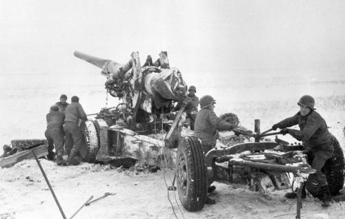
A U.S. M1 155mm towed artillery piece being set up for firing during the Battle of the Bulge, December 1944.
[This series of posts is adapted from the article “Artillery Effectiveness vs. Armor,” by Richard C. Anderson, Jr., originally published in the June 1997 edition of the International TNDM Newsletter.]
The effectiveness of artillery against exposed personnel and other “soft” targets has long been accepted. Fragments and blast are deadly to those unfortunate enough to not be under cover. What has also long been accepted is the relative—if not total—immunity of armored vehicles when exposed to shell fire. In a recent memorandum, the United States Army Armor School disputed the results of tests of artillery versus tanks by stating, “…the Armor School nonconcurred with the Artillery School regarding the suppressive effects of artillery…the M-1 main battle tank cannot be destroyed by artillery…”
This statement may in fact be true,[1] if the advancement of armored vehicle design has greatly exceeded the advancement of artillery weapon design in the last fifty years. [Original emphasis] However, if the statement is not true, then recent research by TDI[2] into the effectiveness of artillery shell fire versus tanks in World War II may be illuminating.
The TDI search found that an average of 12.8 percent of tank and other armored vehicle losses[3] were due to artillery fire in seven eases in World War II where the cause of loss could be reliably identified. The highest percent loss due to artillery was found to be 14.8 percent in the case of the Soviet 1st Tank Army at Kursk (Table II). The lowest percent loss due to artillery was found to be 5.9 percent in the case of Dom Bütgenbach (Table VIII).
The seven cases are split almost evenly between those that show armor losses to a defender and those that show losses to an attacker. The first four cases (Kursk, Normandy l. Normandy ll, and the “Pocket“) are engagements in which the side for which armor losses were recorded was on the defensive. The last three cases (Ardennes, Krinkelt. and Dom Bütgenbach) are engagements in which the side for which armor losses were recorded was on the offensive.
Four of the seven eases (Normandy I, Normandy ll, the “Pocket,” and Ardennes) represent data collected by operations research personnel utilizing rigid criteria for the identification of the cause of loss. Specific causes of loss were only given when the primary destructive agent could be clearly identified. The other three cases (Kursk, Krinkelt, and Dom Bütgenbach) are based upon combat reports that—of necessity—represent less precise data collection efforts.
However, the similarity in results remains striking. The largest identifiable cause of tank loss found in the data was, predictably, high-velocity armor piercing (AP) antitank rounds. AP rounds were found to be the cause of 68.7 percent of all losses. Artillery was second, responsible for 12.8 percent of all losses. Air attack as a cause was third, accounting for 7.4 percent of the total lost. Unknown causes, which included losses due to hits from multiple weapon types as well as unidentified weapons, inflicted 6.3% of the losses and ranked fourth. Other causes, which included infantry antitank weapons and mines, were responsible for 4.8% of the losses and ranked fifth.
NOTES
[1] The statement may be true, although it has an “unsinkable Titanic,” ring to it. It is much more likely that this statement is a hypothesis, rather than a truism.
[2] As pan of this article a survey of the Research Analysis Corporation’s publications list was made in an attempt to locate data from previous operations research on the subject. A single reference to the study of tank losses was found. Group 1 Alvin D. Coox and L. Van Loan Naisawald, Survey of Allied Tank Casualties in World War II, CONFIDENTIAL ORO Report T-117, 1 March 1951.
[3] The percentage loss by cause excludes vehicles lost due to mechanical breakdown or abandonment. lf these were included, they would account for 29.2 percent of the total lost. However, 271 of the 404 (67.1%) abandoned were lost in just two of the cases. These two cases (Normandy ll and the Falaise Pocket) cover the period in the Normandy Campaign when the Allies broke through the German defenses and began the pursuit across France.
Trevor N. Dupuy (1916-1995) and General William E. DePuy (1919-1992)
I first became acquainted with Trevor Dupuy and his work after seeing an advertisement for his book Numbers, Prediction & War in Simulation Publications, Inc.’s (SPI) Strategy & Tactics war gaming magazine way back in the late 1970s. Although Dupuy was already a prolific military historian, this book brought him to the attention of an audience outside of the insular world of the U.S. government military operations research and analysis community.
The two men had a great deal in common. They were born within three years of one another and both served in the U.S. Army during World War II. Both possessed an analytical bent and each made significant contributions to institutional and public debates about combat and warfare in the late 20th century. Given that they tilled the same topical fields at about the same time, it does not seem too odd that they were mistaken for each other.
Perhaps the most enduring link between the two men has been a shared name, though they spelled and pronounced it differently. The surname Dupuy is of medieval French origin and has been traced back to LePuy, France, in the province of Languedoc. It has several variant spellings, including DePuy and Dupuis. The traditional French pronunciation is “do-PWEE.” This is how Trevor Dupuy said his name.
However, following French immigration to North America beginning in the 17th century, the name evolved an anglicized spelling, DePuy (or sometimes Depew), and pronunciation, “deh-PEW.” This is the way General DePuy said it.
It is this pronunciation difference in conversation that has tipped me off personally to the occasional confusion in identities. Though rare these days, it still occurs. While this is a historical footnote, it still seems worth gently noting that Trevor Dupuy and William DePuy were two different people.
Consistent Scoring of Weapons and Aggregation of Forces: The Cornerstone of Dupuy’s Quantitative Analysis of Historical Land Battles by
James G. Taylor, PhD,
Dept. of Operations Research, Naval Postgraduate School
Introduction
Col. Trevor N. Dupuy was an American original, especially as regards the quantitative study of warfare. As with many prophets, he was not entirely appreciated in his own land, particularly its Military Operations Research (OR) community. However, after becoming rather familiar with the details of his mathematical modeling of ground combat based on historical data, I became aware of the basic scientific soundness of his approach. Unfortunately, his documentation of methodology was not always accepted by others, many of whom appeared to confuse lack of mathematical sophistication in his documentation with lack of scientific validity of his basic methodology.
The purpose of this brief paper is to review the salient points of Dupuy’s methodology from a system’s perspective, i.e., to view his methodology as a system, functioning as an organic whole to capture the essence of past combat experience (with an eye towards extrapolation into the future). The advantage of this perspective is that it immediately leads one to the conclusion that if one wants to use some functional relationship derived from Dupuy’s work, then one should use his methodologies for scoring weapons, aggregating forces, and adjusting for operational circumstances; since this consistency is the only guarantee of being able to reproduce historical results and to project them into the future.
Implications (of this system’s perspective on Dupuy’s work) for current DOD models will be discussed. In particular, the Military OR community has developed quantitative methods for imputing values to weapon systems based on their attrition capability against opposing forces and force interactions.[1] One such approach is the so-called antipotential-potential method[2] used in TACWAR[3] to score weapons. However, one should not expect such scores to provide valid casualty estimates when combined with historically derived functional relationships such as the so-called ATLAS casualty-rate curves[4] used in TACWAR, because a different “yard-stick” (i.e. measuring system for estimating the relative combat potential of opposing forces) was used to develop such a curve.
Overview of Dupuy’s Approach
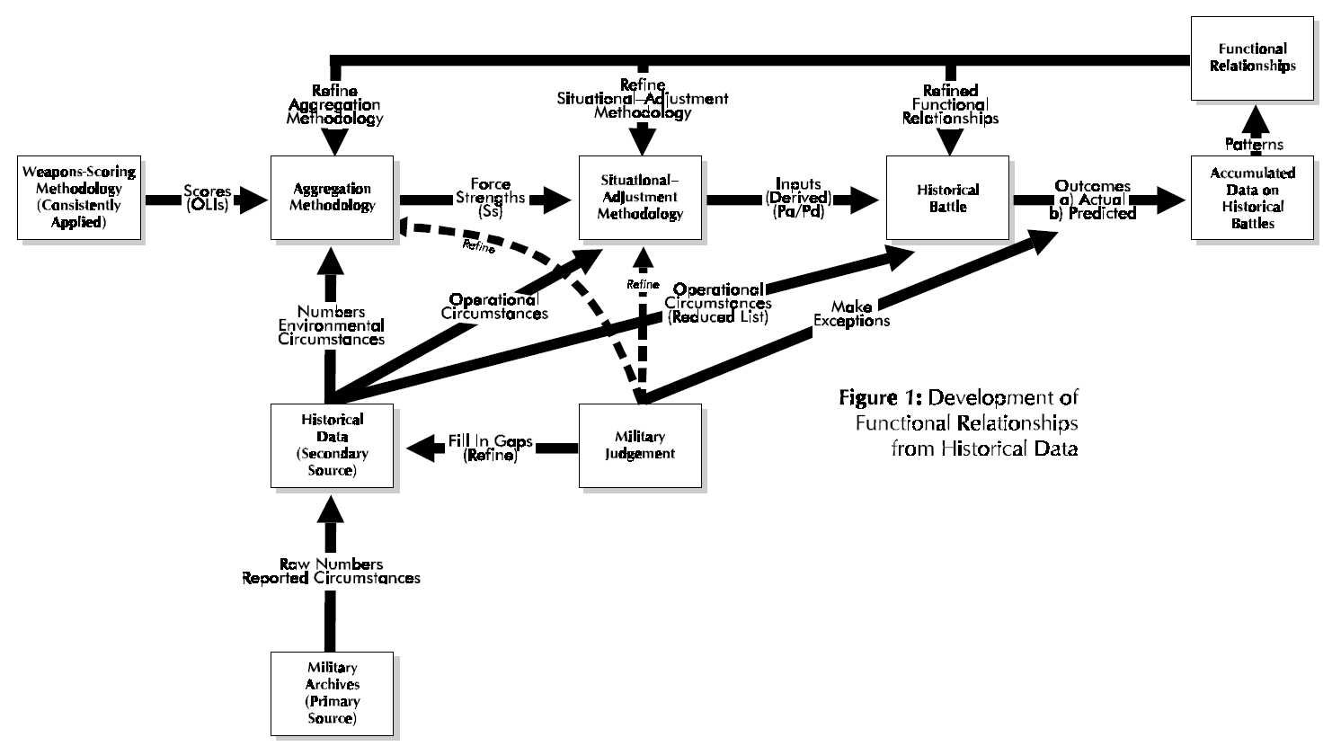
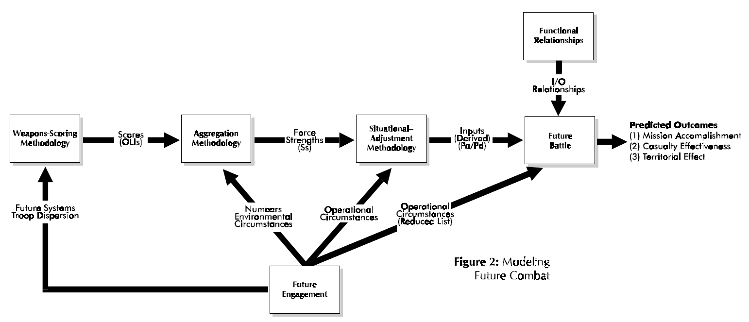
This section briefly outlines the salient features of Dupuy’s approach to the quantitative analysis and modeling of ground combat as embodied in his Tactical Numerical Deterministic Model (TNDM) and its predecessor the Quantified Judgment Model (QJM). The interested reader can find details in Dupuy [1979] (see also Dupuy [1985][5], [1987], [1990]). Here we will view Dupuy’s methodology from a system approach, which seeks to discern its various components and their interactions and to view these components as an organic whole. Essentially Dupuy’s approach involves the development of functional relationships from historical combat data (see Fig. 1) and then using these functional relationships to model future combat (see Fig, 2).
At the heart of Dupuy’s method is the investigation of historical battles and comparing the relationship of inputs (as quantified by relative combat power, denoted as Pa/Pd for that of the attacker relative to that of the defender in Fig. l)(e.g. see Dupuy [1979, pp. 59-64]) to outputs (as quantified by extent of mission accomplishment, casualty effectiveness, and territorial effectiveness; see Fig. 2) (e.g. see Dupuy [1979, pp. 47-50]), The salient point is that within this scheme, the main input[6] (i.e. relative combat power) to a historical battle is a derived quantity. It is computed from formulas that involve three essential aspects: (1) the scoring of weapons (e.g, see Dupuy [1979, Chapter 2 and also Appendix A]), (2) aggregation methodology for a force (e.g. see Dupuy [1979, pp. 43-46 and 202-203]), and (3) situational-adjustment methodology for determining the relative combat power of opposing forces (e.g. see Dupuy [1979, pp. 46-47 and 203-204]). In the force-aggregation step the effects on weapons of Dupuy’s environmental variables and one operational variable (air superiority) are considered[7], while in the situation-adjustment step the effects on forces of his behavioral variables[8] (aggregated into a single factor called the relative combat effectiveness value (CEV)) and also the other operational variables are considered (Dupuy [1987, pp. 86-89])
Figure 1.
Moreover, any functional relationships developed by Dupuy depend (unless shown otherwise) on his computational system for derived quantities, namely OLls, force strengths, and relative combat power. Thus, Dupuy’s results depend in an essential manner on his overall computational system described immediately above. Consequently, any such functional relationship (e.g. casualty-rate curve) directly or indirectly derivative from Dupuy‘s work should still use his computational methodology for determination of independent-variable values.
Fig l also reveals another important aspect of Dupuy’s work, the development of reliable data on historical battles, Military judgment plays an essential role in this development of such historical data for a variety of reasons. Dupuy was essentially the only source of new secondary historical data developed from primary sources (see McQuie [1970] for further details). These primary sources are well known to be both incomplete and inconsistent, so that military judgment must be used to fill in the many gaps and reconcile observed inconsistencies. Moreover, military judgment also generates the working hypotheses for model development (e.g. identification of significant variables).
At the heart of Dupuy’s quantitative investigation of historical battles and subsequent model development is his own weapons-scoring methodology, which slowly evolved out of study efforts by the Historical Evaluation Research Organization (HERO) and its successor organizations (cf. HERO [1967] and compare with Dupuy [1979]). Early HERO [1967, pp. 7-8] work revealed that what one would today call weapons scores developed by other organizations were so poorly documented that HERO had to create its own methodology for developing the relative lethality of weapons, which eventually evolved into Dupuy’s Operational Lethality Indices (OLIs). Dupuy realized that his method was arbitrary (as indeed is its counterpart, called the operational definition, in formal scientific work), but felt that this would be ameliorated if the weapons-scoring methodology be consistently applied to historical battles. Unfortunately, this point is not clearly stated in Dupuy’s formal writings, although it was clearly (and compellingly) made by him in numerous briefings that this author heard over the years.
Figure 2.
In other words, from a system’s perspective, the functional relationships developed by Colonel Dupuy are part of his analysis system that includes this weapons-scoring methodology consistently applied (see Fig. l again). The derived functional relationships do not stand alone (unless further empirical analysis shows them to hold for any weapons-scoring methodology), but function in concert with computational procedures. Another essential part of this system is Dupuy‘s aggregation methodology, which combines numbers, environmental circumstances, and weapons scores to compute the strength (S) of a military force. A key innovation by Colonel Dupuy [1979, pp. 202- 203] was to use a nonlinear (more precisely, a piecewise-linear) model for certain elements of force strength. This innovation precluded the occurrence of military absurdities such as air firepower being fully substitutable for ground firepower, antitank weapons being fully effective when armor targets are lacking, etc‘ The final part of this computational system is Dupuy’s situational-adjustment methodology, which combines the effects of operational circumstances with force strengths to determine relative combat power, e.g. Pa/Pd.
To recapitulate, the determination of an Operational Lethality Index (OLI) for a weapon involves the combination of weapon lethality, quantified in terms of a Theoretical Lethality Index (TLI) (e.g. see Dupuy [1987, p. 84]), and troop dispersion[9] (e.g. see Dupuy [1987, pp. 84- 85]). Weapons scores (i.e. the OLIs) are then combined with numbers (own side and enemy) and combat- environment factors to yield force strength. Six[10] different categories of weapons are aggregated, with nonlinear (i.e. piecewise-linear) models being used for the following three categories of weapons: antitank, air defense, and air firepower (i.e. c1ose—air support). Operational, e.g. mobility, posture, surprise, etc. (Dupuy [1987, p. 87]), and behavioral variables (quantified as a relative combat effectiveness value (CEV)) are then applied to force strength to determine a side’s combat-power potential.
Requirement for Consistent Scoring of Weapons, Force Aggregation, and Situational Adjustment for Operational Circumstances
The salient point to be gleaned from Fig.1 and 2 is that the same (or at least consistent) weapons—scoring, aggregation, and situational—adjustment methodologies be used for both developing functional relationships and then playing them to model future combat. The corresponding computational methods function as a system (organic whole) for determining relative combat power, e.g. Pa/Pd. For the development of functional relationships from historical data, a force ratio (relative combat power of the two opposing sides, e.g. attacker’s combat power divided by that of the defender, Pa/Pd is computed (i.e. it is a derived quantity) as the independent variable, with observed combat outcome being the dependent variable. Thus, as discussed above, this force ratio depends on the methodologies for scoring weapons, aggregating force strengths, and adjusting a force’s combat power for the operational circumstances of the engagement. It is a priori not clear that different scoring, aggregation, and situational-adjustment methodologies will lead to similar derived values. If such different computational procedures were to be used, these derived values should be recomputed and the corresponding functional relationships rederived and replotted.
However, users of the Tactical Numerical Deterministic Model (TNDM) (or for that matter, its predecessor, the Quantified Judgment Model (QJM)) need not worry about this point because it was apparently meticulously observed by Colonel Dupuy in all his work. However, portions of his work have found their way into a surprisingly large number of DOD models (usually not explicitly acknowledged), but the context and range of validity of historical results have been largely ignored by others. The need for recalibration of the historical data and corresponding functional relationships has not been considered in applying Dupuy’s results for some important current DOD models.
Implications for Current DOD Models
A number of important current DOD models (namely, TACWAR and JICM discussed below) make use of some of Dupuy’s historical results without recalibrating functional relationships such as loss rates and rates of advance as a function of some force ratio (e.g. Pa/Pd). As discussed above, it is not clear that such a procedure will capture the essence of past combat experience. Moreover, in calculating losses, Dupuy first determines personnel losses (expressed as a percent loss of personnel strength, i.e., number of combatants on a side) and then calculates equipment losses as a function of this casualty rate (e.g., see Dupuy [1971, pp. 219-223], also [1990, Chapters 5 through 7][11]). These latter functional relationships are apparently not observed in the models discussed below. In fact, only Dupuy (going back to Dupuy [1979][12] takes personnel losses to depend on a force ratio and other pertinent variables, with materiel losses being taken as derivative from this casualty rate.
For example, TACWAR determines personnel losses[13] by computing a force ratio and then consulting an appropriate casualty-rate curve (referred to as empirical data), much in the same fashion as ATLAS did[14]. However, such a force ratio is computed using a linear model with weapon values determined by the so-called antipotential-potential method[15]. Unfortunately, this procedure may not be consistent with how the empirical data (i.e. the casualty-rate curves) was developed. Further research is required to demonstrate that valid casualty estimates are obtained when different weapon scoring, aggregation, and situational-adjustment methodologies are used to develop casualty-rate curves from historical data and to use them to assess losses in aggregated combat models. Furthermore, TACWAR does not use Dupuy’s model for equipment losses (see above), although it does purport, as just noted above, to use “historical data” (e.g., see Kerlin et al. [1975, p. 22]) to compute personnel losses as a function (among other things) of a force ratio (given by a linear relationship), involving close air support values in a way never used by Dupuy. Although their force-ratio determination methodology does have logical and mathematical merit, it is not the way that the historical data was developed.
Moreover, RAND (Allen [1992]) has more recently developed what is called the situational force scoring (SFS) methodology for calculating force ratios in large-scale, aggregated-force combat situations to determine loss and movement rates. Here, SFS refers essentially to a force- aggregation and situation-adjustment methodology, which has many conceptual elements in common with Dupuy‘s methodology (except, most notably, extensive testing against historical data, especially documentation of such efforts). This SFS was originally developed for RSAS[16] and is today used in JICM[17]. It also apparently uses a weapon-scoring system developed at RAND[18]. It purports (no documentation given [citation of unpublished work]) to be consistent with historical data (including the ATLAS casualty-rate curves) (Allen [1992, p.41]), but again no consideration is given to recalibration of historical results for different weapon scoring, force-aggregation, and situational-adjustment methodologies. SFS emphasizes adjusting force strengths according to operational circumstances (the “situation”) of the engagement (including surprise), with many innovative ideas (but in some major ways has little connection with previous work of others[19]). The resulting model contains many more details than historical combat data would support. It also is methodology that differs in many essential ways from that used previously by any investigator. In particular, it is doubtful that it develops force ratios in a manner consistent with Dupuy’s work.
Final Comments
Use of (sophisticated) mathematics for modeling past historical combat (and extrapolating it into the future for planning purposes) is no reason for ignoring Dupuy’s work. One would think that the current Military OR community would try to understand Dupuy’s work before trying to improve and extend it. In particular, Colonel Dupuy’s various computational procedures (including constants) must be considered as an organic whole (i.e. a system) supporting the development of functional relationships. If one ignores this computational system and simply tries to use some isolated aspect, the result may be interesting and even logically sound, but it probably lacks any scientific validity.
REFERENCES
P. Allen, “Situational Force Scoring: Accounting for Combined Arms Effects in Aggregate Combat Models,” N-3423-NA, The RAND Corporation, Santa Monica, CA, 1992.
L. B. Anderson, “A Briefing on Anti-Potential Potential (The Eigen-value Method for Computing Weapon Values), WP-2, Project 23-31, Institute for Defense Analyses, Arlington, VA, March 1974.
B. W. Bennett, et al, “RSAS 4.6 Summary,” N-3534-NA, The RAND Corporation, Santa Monica, CA, 1992.
B. W. Bennett, A. M. Bullock, D. B. Fox, C. M. Jones, J. Schrader, R. Weissler, and B. A. Wilson, “JICM 1.0 Summary,” MR-383-NA, The RAND Corporation, Santa Monica, CA, 1994.
P. K. Davis and J. A. Winnefeld, “The RAND Strategic Assessment Center: An Overview and Interim Conclusions About Utility and Development Options,” R-2945-DNA, The RAND Corporation, Santa Monica, CA, March 1983.
T.N, Dupuy, Numbers. Predictions and War: Using History to Evaluate Combat Factors and Predict the Outcome of Battles, The Bobbs-Merrill Company, Indianapolis/New York, 1979,
T.N. Dupuy, Numbers Predictions and War, Revised Edition, HERO Books, Fairfax, VA 1985.
T.N. Dupuy, Understanding War: History and Theory of Combat, Paragon House Publishers, New York, 1987.
T.N. Dupuy, Attrition: Forecasting Battle Casualties and Equipment Losses in Modem War, HERO Books, Fairfax, VA, 1990.
General Research Corporation (GRC), “A Hierarchy of Combat Analysis Models,” McLean, VA, January 1973.
Historical Evaluation and Research Organization (HERO), “Average Casualty Rates for War Games, Based on Historical Data,” 3 Volumes in 1, Dunn Loring, VA, February 1967.
E. P. Kerlin and R. H. Cole, “ATLAS: A Tactical, Logistical, and Air Simulation: Documentation and User’s Guide,” RAC-TP-338, Research Analysis Corporation, McLean, VA, April 1969 (AD 850 355).
E.P. Kerlin, L.A. Schmidt, A.J. Rolfe, M.J. Hutzler, and D,L. Moody, “The IDA Tactical Warfare Model: A Theater-Level Model of Conventional, Nuclear, and Chemical Warfare, Volume II- Detailed Description” R-21 1, Institute for Defense Analyses, Arlington, VA, October 1975 (AD B009 692L).
R. McQuie, “Military History and Mathematical Analysis,” Military Review 50, No, 5, 8-17 (1970).
S.M. Robinson, “Shadow Prices for Measures of Effectiveness, I: Linear Model,” Operations Research 41, 518-535 (1993).
J.G. Taylor, Lanchester Models of Warfare. Vols, I & II. Operations Research Society of America, Alexandria, VA, 1983. (a)
J.G. Taylor, “A Lanchester-Type Aggregated-Force Model of Conventional Ground Combat,” Naval Research Logistics Quarterly 30, 237-260 (1983). (b)
NOTES
[1] For example, see Taylor [1983a, Section 7.18], which contains a number of examples. The basic references given there may be more accessible through Robinson [I993].
[2] This term was apparently coined by L.B. Anderson [I974] (see also Kerlin et al. [1975, Chapter I, Section D.3]).
[3] The Tactical Warfare (TACWAR) model is a theater-level, joint-warfare, computer-based combat model that is currently used for decision support by the Joint Staff and essentially all CINC staffs. It was originally developed by the Institute for Defense Analyses in the mid-1970s (see Kerlin et al. [1975]), originally referred to as TACNUC, which has been continually upgraded until (and including) the present day.
[4] For example, see Kerlin and Cole [1969], GRC [1973, Fig. 6-6], or Taylor [1983b, Fig. 5] (also Taylor [1983a, Section 7.13]).
[5] The only apparent difference between Dupuy [1979] and Dupuy [1985] is the addition of an appendix (Appendix C “Modified Quantified Judgment Analysis of the Bekaa Valley Battle”) to the end of the latter (pp. 241-251). Hence, the page content is apparently the same for these two books for pp. 1-239.
[6] Technically speaking, one also has the engagement type and possibly several other descriptors (denoted in Fig. 1 as reduced list of operational circumstances) as other inputs to a historical battle.
[7] In Dupuy [1979, e.g. pp. 43-46] only environmental variables are mentioned, although basically the same formulas underlie both Dupuy [1979] and Dupuy [1987]. For simplicity, Fig. 1 and 2 follow this usage and employ the term “environmental circumstances.”
[8] In Dupuy [1979, e.g. pp. 46-47] only operational variables are mentioned, although basically the same formulas underlie both Dupuy [1979] and Dupuy [1987]. For simplicity, Fig. 1 and 2 follow this usage and employ the term “operational circumstances.”
[9] Chris Lawrence has kindly brought to my attention that since the same value for troop dispersion from an historical period (e.g. see Dupuy [1987, p. 84]) is used for both the attacker and also the defender, troop dispersion does not actually affect the determination of relative combat power PM/Pd.
[10] Eight different weapon types are considered, with three being classified as infantry weapons (e.g. see Dupuy [1979, pp, 43-44], [1981 pp. 85-86]).
[11] Chris Lawrence has kindly informed me that Dupuy‘s work on relating equipment losses to personnel losses goes back to the early 1970s and even earlier (e.g. see HERO [1966]). Moreover, Dupuy‘s [1992] book Future Wars gives some additional empirical evidence concerning the dependence of equipment losses on casualty rates.
[12] But actually going back much earlier as pointed out in the previous footnote.
[13] See Kerlin et al. [1975, Chapter I, Section D.l].
[14] See Footnote 4 above.
[15] See Kerlin et al. [1975, Chapter I, Section D.3]; see also Footnotes 1 and 2 above.
[16] The RAND Strategy Assessment System (RSAS) is a multi-theater aggregated combat model developed at RAND in the early l980s (for further details see Davis and Winnefeld [1983] and Bennett et al. [1992]). It evolved into the Joint Integrated Contingency Model (JICM), which is a post-Cold War redesign of the RSAS (starting in FY92).
[17] The Joint Integrated Contingency Model (JICM) is a game-structured computer-based combat model of major regional contingencies and higher-level conflicts, covering strategic mobility, regional conventional and nuclear warfare in multiple theaters, naval warfare, and strategic nuclear warfare (for further details, see Bennett et al. [1994]).
[18] RAND apparently replaced one weapon-scoring system by another (e.g. see Allen [1992, pp. 9, l5, and 87-89]) without making any other changes in their SFS System.
[19] For example, both Dupuy’s early HERO work (e.g. see Dupuy [1967]), reworks of these results by the Research Analysis Corporation (RAC) (e.g. see RAC [1973, Fig. 6-6]), and Dupuy’s later work (e.g. see Dupuy [1979]) considered daily fractional casualties for the attacker and also for the defender as basic casualty-outcome descriptors (see also Taylor [1983b]). However, RAND does not do this, but considers the defender’s loss rate and a casualty exchange ratio as being the basic casualty-production descriptors (Allen [1992, pp. 41-42]). The great value of using the former set of descriptors (i.e. attacker and defender fractional loss rates) is that not only is casualty assessment more straight forward (especially development of functional relationships from historical data) but also qualitative model behavior is readily deduced (see Taylor [1983b] for further details).
In 1931, Lieutenant Colonel (later Brigadier General) Love, then a Medical Corps physician in the U.S. Army Medical Field Services School, published a study of American casualty data in the recent Great War, titled “War Casualties.”[1] This study was likely the source for tables used for casualty estimation by the U.S. Army through 1944.[2]
Love’s research was likely the basis for rate tables for calculating casualties that first appeared in the 1932 edition of the War Department’s Staff Officer’s Field Manual.[3]
Battle Casualties, including Killed, in Percent of Unit Strength, Staff Officer’s Field Manual (1932).
The 1932 Staff Officer’s Field Manual estimation methodology reflected Love’s sophisticated understanding of the factors influencing combat casualty rates. It showed that both the resistance and combat strength (and all of the factors that comprised it) of the enemy, as well as the equipment and state of training and discipline of the friendly troops had to be taken into consideration. The text accompanying the tables pointed out that loss rates in small units could be quite high and variable over time, and that larger formations took fewer casualties as a fraction of overall strength, and that their rates tended to become more constant over time. Casualties were not distributed evenly, but concentrated most heavily among the combat arms, and in the front-line infantry in particular. Attackers usually suffered higher loss rates than defenders. Other factors to be accounted for included the character of the terrain, the relative amount of artillery on each side, and the employment of gas.
The 1941 iteration of the Staff Officer’s Field Manual, now designated Field Manual (FM) 101-10[4], provided two methods for estimating battle casualties. It included the original 1932 Battle Casualties table, but the associated text no longer included the section outlining factors to be considered in calculating loss rates. This passage was moved to a note appended to a new table showing the distribution of casualties among the combat arms.
Rather confusingly, FM 101-10 (1941) presented a second table, Estimated Daily Losses in Campaign of Personnel, Dead and Evacuated, Per 1,000 of Actual Strength. It included rates for front line regiments and divisions, corps and army units, reserves, and attached cavalry. The rates were broken down by posture and tactical mission.
Estimated Daily Losses in Campaign of Personnel, Dead and Evacuated, Per 1,000 of Actual Strength, FM 101-10 (1941)
The source for this table is unknown, nor the method by which it was derived. No explanatory text accompanied it, but a footnote stated that “this table is intended primarily for use in school work and in field exercises.” The rates in it were weighted toward the upper range of the figures provided in the 1932 Battle Casualties table.
The October 1943 edition of FM 101-10 contained no significant changes from the 1941 version, except for the caveat that the 1932 Battle Casualties table “may or may not prove correct when applied to the present conflict.”
The October 1944 version of FM 101-10 incorporated data obtained from World War II experience.[5] While it also noted that the 1932 Battle Casualties table might not be applicable, the experiences of the U.S. II Corps in North Africa and one division in Italy were found to be in agreement with the table’s division and corps loss rates.
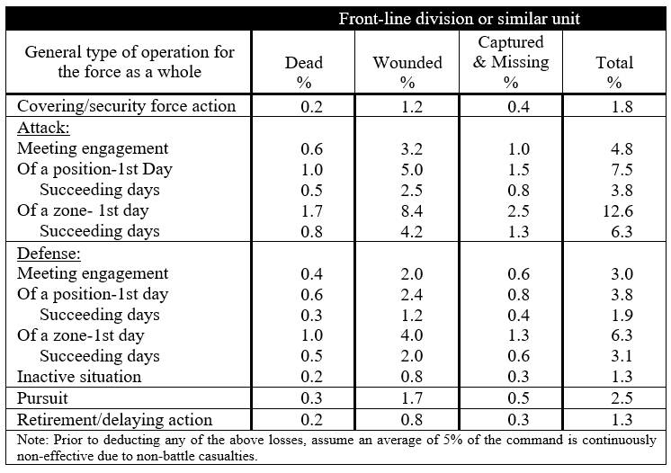
FM 101-10 (1944) included another new table, Estimate of Battle Losses for a Front-Line Division (in % of Actual Strength), meaning that it now provided three distinct methods for estimating battle casualties.
Estimate of Battle Losses for a Front-Line Division (in % of Actual Strength), FM 101-10 (1944)
Like the 1941 Estimated Daily Losses in Campaign table, the sources for this new table were not provided, and the text contained no guidance as to how or when it should be used. The rates it contained fell roughly within the span for daily rates for severe (6-8%) to maximum (12%) combat listed in the 1932 Battle Casualty table, but would produce vastly higher overall rates if applied consistently, much higher than the 1932 table’s 1% daily average.
FM 101-10 (1944) included a table showing the distribution of losses by branch for the theater based on experience to that date, except for combat in the Philippine Islands. The new chart was used in conjunction with the 1944 Estimate of Battle Losses for a Front-Line Division table to determine daily casualty distribution.
Distribution of Battle Losses–Theater of Operations, FM 101-10 (1944)
The final World War II version of FM 101-10 issued in August 1945[6] contained no new casualty rate tables, nor any revisions to the existing figures. It did finally effectively invalidate the 1932 Battle Casualties table by noting that “the following table has been developed from American experience in active operations and, of course, may not be applicable to a particular situation.” (original emphasis)
NOTES
[1] Albert G. Love, War Casualties, The Army Medical Bulletin, No. 24, (Carlisle Barracks, PA: 1931)
[2] This post is adapted from TDI, Casualty Estimation Methodologies Study, Interim Report (May 2005) (Altarum) (pp. 314-317).
[3] U.S. War Department, Staff Officer’s Field Manual, Part Two: Technical and Logistical Data (Government Printing Office, Washington, D.C., 1932)
[4] U.S. War Department, FM 101-10, Staff Officer’s Field Manual: Organization, Technical and Logistical Data (Washington, D.C., June 15, 1941)
[5] U.S. War Department, FM 101-10, Staff Officer’s Field Manual: Organization, Technical and Logistical Data (Washington, D.C., October 12, 1944)
[6] U.S. War Department, FM 101-10 Staff Officer’s Field Manual: Organization, Technical and Logistical Data (Washington, D.C., August 1, 1945)
Stretcher bearers of the East Surrey Regiment, with a Churchill tank of the North Irish Horse in the background, during the attack on Longstop Hill, Tunisia, 23 April 1943. [Imperial War Museum/Wikimedia]
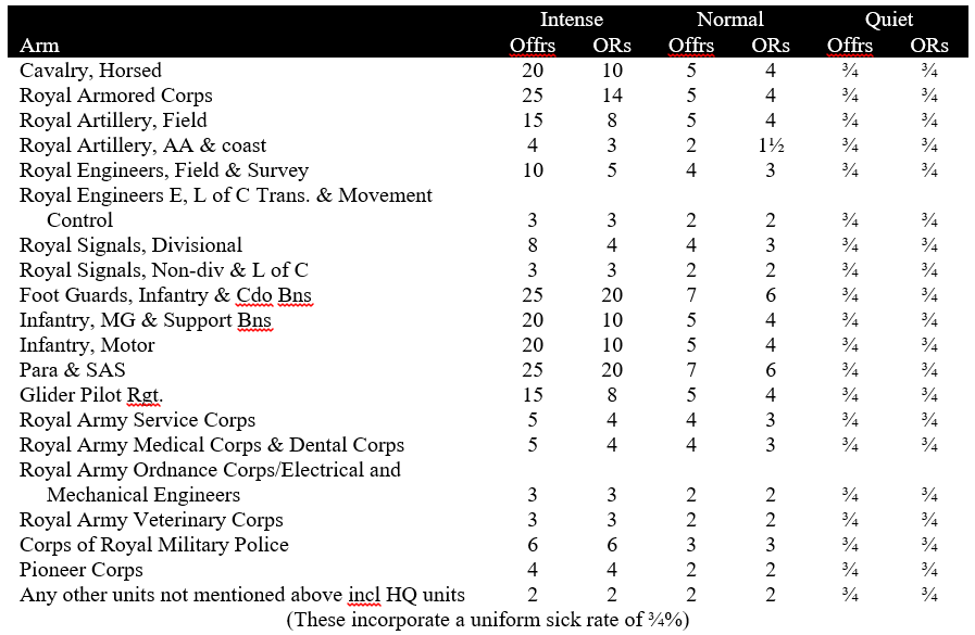
British Army staff officers during World War II and the 1950s used a set of look-up tables which listed expected monthly losses in percentage of strength for various arms under various combat conditions. The origin of the tables is not known, but they were officially updated twice, in 1942 by a committee chaired by Major General Evett, and in 1951-1955 by the Army Operations Research Group (AORG).[2]
The methodology was based on staff predictions of one of three levels of operational activity, “Intense,” “Normal,” and “Quiet.” These could be applied to an entire theater, or to individual divisions. The three levels were defined the same way for both the Evett Committee and AORG rates:
The rates were broken down by arm and rank, and included battle and nonbattle casualties.
Rates of Personnel Wastage Including Both Battle and Non-battle Casualties According to the Evett Committee of 1942. (Percent per 30 days).
The Evett Committee rates were criticized during and after the war. After British forces suffered twice the anticipated casualties at Anzio, the British 21st Army Group applied a “double intense rate” which was twice the Evett Committee figure and intended to apply to assaults. When this led to overestimates of casualties in Normandy, the double intense rate was discarded.
From 1951 to 1955, AORG undertook a study of casualty rates in World War II. Its analysis was based on casualty data from the following campaigns:
Northwest Europe, 1944
6-30 June – Beachhead offensive
1 July-1 September – Containment and breakout
1 October-30 December – Semi-static phase
9 February to 6 May – Rhine crossing and final phase
Italy, 1944
January to December – Fighting a relatively equal enemy in difficult country. Warfare often static.
January to February (Anzio) – Beachhead held against severe and well-conducted enemy counter-attacks.
North Africa, 1943
14 March-13 May – final assault
Northwest Europe, 1940
10 May-2 June – Withdrawal of BEF
Burma, 1944-45
From the first four cases, the AORG study calculated two sets of battle casualty rates as percentage of strength per 30 days. “Overall” rates included KIA, WIA, C/MIA. “Apparent rates” included these categories but subtracted troops returning to duty. AORG recommended that “overall” rates be used for the first three months of a campaign.
The Burma campaign data was evaluated differently. The analysts defined a “force wastage” category which included KIA, C/MIA, evacuees from outside the force operating area and base hospitals, and DNBI deaths. “Dead wastage” included KIA, C/MIA, DNBI dead, and those discharged from the Army as a result of injuries.
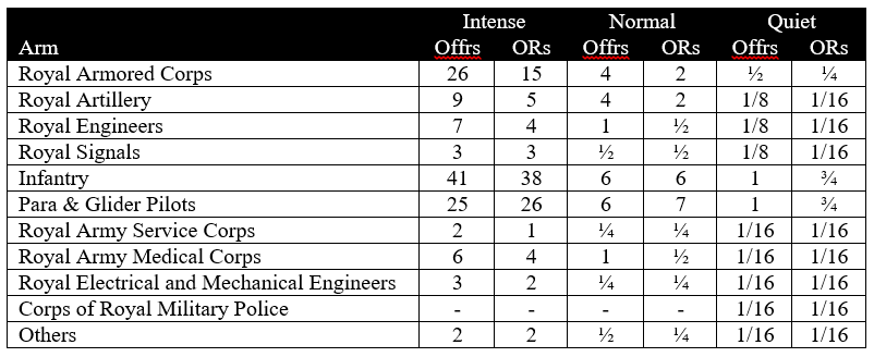
The AORG study concluded that the Evett Committee underestimated intense loss rates for infantry and armor during periods of very hard fighting and overestimated casualty rates for other arms. It recommended that if only one brigade in a division was engaged, two-thirds of the intense rate should be applied, if two brigades were engaged the intense rate should be applied, and if all brigades were engaged then the intense rate should be doubled. It also recommended that 2% extra casualties per month should be added to all the rates for all activities should the forces encounter heavy enemy air activity.[1]
The AORG study rates were as follows:
Recommended AORG Rates of Personnel Wastage. (Percent per 30 days).
If anyone has further details on the origins and activities of the Evett Committee and AORG, we would be very interested in finding out more on this subject.
NOTES
[1] This post is adapted from The Dupuy Institute, Casualty Estimation Methodologies Study, Interim Report (May 2005) (Altarum) (pp. 51-53).
[2] Rowland Goodman and Hugh Richardson. “Casualty Estimation in Open and Guerrilla Warfare.” (London: Directorate of Science (Land), U.K. Ministry of Defence, June 1995.), Appendix A.
Trevor Dupuy distilled his research and analysis on combat into a series of verities, or what he believed were empirically-derived principles. He intended for his verities to complement the classic principles of war, a slightly variable list of maxims of unknown derivation and provenance, which describe the essence of warfare largely from the perspective of Western societies. These are summarized below.
Over the years I have run across a number of Australian Operations Research and Historical Analysis efforts. Overall, I have been impressed with what I have seen. Below is one of their papers written by Nigel Perry. He is not otherwise known to me. It is dated December 2011: Applications of Historical Analyses in Combat Modeling
It does address the value of Lanchester equations in force-on-force combat models, which in my mind is already a settled argument (see: Lanchester Equations Have Been Weighed). His is the latest argument that I gather reinforces this point.
The author of this paper references the work of Robert Helmbold and Dean Hartley (see page 14). He does favorably reference the work of Trevor Dupuy but does not seem to be completely aware of the extent or full nature of it (pages 14, 16, 17, 24 and 53). He does not seem to aware that the work of Helmbold and Hartley was both built from a database that was created by Trevor Dupuy’s companies HERO & DMSI. Without Dupuy, Helmbold and Hartley would not have had data to work from.
Specifically, Helmbold was using the Chase database, which was programmed by the government from the original paper version provided by Dupuy. I think it consisted of 597-599 battles (working from memory here). It also included a number of coding errors when they programmed it and did not include the battle narratives. Hartley had Oakridge National Laboratories purchase a computerized copy from Dupuy of what was now called the Land Warfare Data Base (LWDB). It consisted of 603 or 605 engagements (and did not have the coding errors but still did not include the narratives). As such, they both worked from almost the same databases.
Dr. Perrty does take a copy of Hartley’s database and expands it to create more engagements. He says he expanded it from 750 battles (except the database we sold to Harley had 603 or 605 cases) to around 1600. It was estimated in the 1980s by Curt Johnson (Director and VP of HERO) to take three man-days to create a battle. If this estimate is valid (actually I think it is low), then to get to 1600 engagements the Australian researchers either invested something like 10 man-years of research, or relied heavily on secondary sources without any systematic research, or only partly developed each engagement (for example, only who won and lost). I suspect the latter.
Post WWII………….1950……..2008…………118……………….86…………….32
We, of course, did something very similar. We took the Land Warfare Data Base (the 605 engagement version), expanded in considerably with WWII and post-WWII data, proofed and revised a number of engagements using more primarily source data, divided it into levels of combat (army-level, division-level, battalion-level, company-level) and conducted analysis with the 1280 or so engagements we had. This was a much more powerful and better organized tool. We also looked at winner and loser, but used the 605 engagement version (as we did the analysis in 1996). An example of this, from pages 16 and 17 of my manuscript for War by Numbers shows:
Attacker Won:
Force Ratio Force Ratio Percent Attack Wins:
Greater than or less than Force Ratio Greater Than
equal to 1-to-1 1-to1 or equal to 1-to-1
1600-1699 16 18 47%
1700-1799 25 16 61%
1800-1899 47 17 73%
1900-1920 69 13 84%
1937-1945 104 8 93%
1967-1973 17 17 50%
Total 278 89 76%
Defender Won:
Force Ratio Force Ratio Percent Defense Wins:
Greater than or less than Force Ratio Greater Than
equal to 1-to-1 1-to1 or equal to 1-to-1
1600-1699 7 6 54%
1700-1799 11 13 46%
1800-1899 38 20 66%
1900-1920 30 13 70%
1937-1945 33 10 77%
1967-1973 11 5 69%
Total 130 67 66%
Anyhow, from there (pages 26-59) the report heads into an extended discussion of the analysis done by Helmbold and Hartley (which I am not that enamored with). My book heads in a different direction: War by Numbers III (Table of Contents)
He actually tested his equations to historical data, which are presented in his paper. He ended up coming up with something similar to Lanchester equations but it did not have a square law, but got a similar effect by putting things to the 3/2nds power.
As far as we know, because of the time it was published (June-October 1915), it was not influenced or done with any awareness of work that the far more famous Frederick Lanchester had done (and Lanchester was famous for a lot more than just his modeling equations). Lanchester first published his work in the fall of 1914 (after the Great War had already started). It is possible that Osipov was aware of it, but he does not mention Lanchester. He was probably not aware of Lanchester’s work. It appears to be the case of him independently coming up with the use of differential equations to describe combat attrition. This was also the case with Rear Admiral J. V. Chase, who wrote a classified staff paper for U.S. Navy in 1902 that was not revealed until 1972.
Osipov, after he had written his paper, may have served in World War I, which was already underway at the time it was published. Between the war, the Russian revolutions, the civil war afterwards, the subsequent repressions by Cheka and later Stalin, we do not know what happened to M. Osipov. At the time I was asked by CAA if our Russian research team knew about him. I passed the question to Col. Sverdlov and Col. Vainer and they were not aware of him. It is probably possible to chase him down, but would probably take some effort. Perhaps some industrious researcher will find out more about him.
It does not appear that Osipov had any influence on Soviet operations research or military analysis. It appears that he was ignored or forgotten. His article was re-published in the September 1988 of the Soviet Military-Historical Journal with the propaganda influenced statement that they also had their own “Lanchester.” Of course, this “Soviet Lanchester” was publishing in a Tsarist military journal, hardly a demonstration of the strength of the Soviet system.
There have been a number of tests of Lanchester equations to historical data over the years. Versions of Lanchester equations were implemented in various ground combat models in the late 1960s and early 1970s without any rigorous testing. As John Stockfish of RAND stated in 1975 in his report: Models, Data, and War: A Critique of the Study of Conventional Forces:
However Lanchester is presently esteemed for his ‘combat model,’ and specifically his ‘N-square law’ of combat, which is nothing more than a mathematical formulation of the age-old military principal of force concentration. That there is no clear empirical verification of this law, or that Lanchester’s model or present versions of it may in fact be incapable of verification, have not detracted from this source of his luster.”
Since John Stockfish’s report in 1975 the tests of Lanchester have included:
(1) Janice B. Fain, “The Lanchester Equations and Historical Warfare: An Analysis of Sixty World War II Land Engagements.” Combat Data Subscription Service (HERO, Arlington, VA, Spring 1977);
(2) D. S. Hartley and R. L. Helmbold, “Validating Lanchester’s Square Law and Other Attrition Models,” in Warfare Modeling, J. Bracken, M. Kress, and R. E. Rosenthal, ed., (New York: John Wiley & Sons, 1995) and originally published in 1993;
(3) Jerome Bracken, “Lanchester Models of the Ardennes Campaign in Warfare Modeling (John Wiley & sons, Danvers, MA, 1995);
(4) R. D. Fricker, “Attrition Models of the Ardennes Campaign,” Naval Research Logistics, vol. 45, no. 1, January 1997;
(5) S. C. Clemens, “The Application of Lanchester Models to the Battle of Kursk” (unpublished manuscript, May 1997);
(6) 1LT Turker Turkes, Turkish Army, “Fitting Lanchester and Other Equations to the Battle of Kursk Data,” Dissertation for MS in Operations Research, March 2000;
(7) Captain John Dinges, U.S. Army, “Exploring the Validation of Lanchester Equations for the Battle of Kursk,” MS in Operations Research, June 2001;
(8) Tom Lucas and Turker Turkes, “Fitting Lanchester Equations to the Battles of Kursk and Ardennes,” Naval Research Logistics, 51, February 2004, pp. 95-116;
(9) Thomas W. Lucas and John A. Dinges, “The Effect of Battle Circumstances on Fitting Lanchester Equations to the Battle of Kursk,” forthcoming in Military Operations Research.
In all cases, it was from different data sets developed by us, with eight of the tests conducted completely independently of us and without our knowledge.
In all cases, they could not establish a Lanchester square law and really could not establish the Lanchester linear law. That is nine separate and independent tests in a row with basically no result. Furthermore, there has never been a test to historical data (meaning real-world combat data) that establishes Lanchester does apply to ground combat. This is added to the fact that Lanchester himself did not think it should. It does not get any clearer than that.
As Morse & Kimball stated in 1951 in Methods of Operations Research
Occasionally, however, it is useful to insert these constants into differential equations, to see what would happen in the long run if conditions were to remain the same, as far as the constants go. These differential equations, in order to be soluble, will have to represent extremely simplified forms of warfare; and therefore their range of applicability will be small.
And later they state:
Indeed an important problem in operations research for any type of warfare is the investigation, both theoretical and statistical, as to how nearly Lanchester’s laws apply.
I think this has now been done for land warfare, at last. Therefore, I conclude: Lanchester equations have been weighed, they have been measured, and they have been found wanting.
RAND described the combat system from their hex boardgame as such:
The general game design was similar to that of traditional board wargames, with a hex grid governing movement superimposed on a map. Tactical Pilotage Charts (1:500,000 scale) were used, overlaid with 10-km hexes, as seen in Figure A.1. Land forces were represented at the battalion level and air units as squadrons; movement and combat were governed and adjudicated using rules and combat-result tables that incorporated both traditional gaming principles (e.g., Lanchester exchange rates) and the results of offline modeling….”
Now this catches my attention. Switching from a “series of tubes” to a hexagon boardgame brings back memories, but it is understandable. On the other hand, it is pretty widely known that no one has been able to make Lanchester equations work when tested to historical ground combat. There have been multiple efforts conducted to test this, mostly using the Ardennes and Kursk databases that we developed. In particular, Jerome Braken published his results in Modeling Warfare and Dr. Thomas Lucas out at Naval Post-Graduate School has conducted multiple tests to try to do the same thing. They all point to the same conclusion, which is that Lanchester equations do not really work for ground combat. They might work for air, but it is hard to tell from the RAND write-up whether they restricted the use of “Lanchester exchange rates” to only air combat. I could make the point by referencing many of these studies but this would be a long post. The issue is briefly discussed in Chapter Eighteen of my upcoming book War by Numbers and is discussed in depth in the TDI report “Casualty Estimation Methodologies Study.” Instead I will leave it to Frederick Lanchester himself, writing in 1914, to summarize the problem:
We have already seen that the N-square law applies broadly, if imperfectly, to military operations. On land, however, there sometimes exist special conditions and a multitude of factors extraneous to the hypothesis, whereby its operations may be suspended or masked.