Tag conventional warfare

Validating A Combat Model (Part VI)

Advancing Germans halted by 2nd Battalion, Fifth Marine, June 3 1918. Les Mares form 2 1/2 miles west of Belleau Wood attacked the American lines through the wheat fields. From a painting by Harvey Dunn. [U.S. Navy]

[The article below is reprinted from April 1997 edition of The International TNDM Newsletter.]

The First Test of the TNDM Battalion-Level Validations: Predicting the Winners
by Christopher A. Lawrence

CASE STUDIES: WHERE AND WHY THE MODEL FAILED CORRECT PREDICTIONS

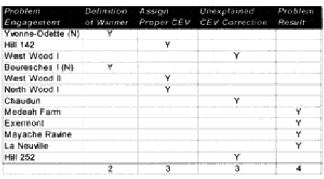
World War I (12 cases):

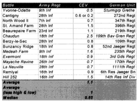
Yvonne-Odette (Night)—On the first prediction, selected the defender as a winner, with the attacker making no advance. The force ratio was 0.5 to 1. The historical results also show e attacker making no advance, but rate the attacker’s mission accomplishment score as 6 while the defender is rated 4. Therefore, this battle was scored as a draw.

On the second run, the Germans (Sturmgruppe Grethe) were assigned a CEV of 1.9 relative to the US 9th Infantry Regiment. This produced a draw with no advance.

This appears to be a result that was corrected by assigning the CEV to the side that would be expected to have that advantage. There is also a problem in defining who is winner.

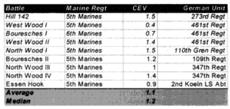
Hill 142—On the first prediction the defending Germans won, whereas in the real world the attacking Marines won. The Marines are recorded as having a higher CEV in a number of battles, so when this correction is put in the Marines win with a CEV of 1.5. This appears to be a case where the side that would be expected to have the higher CEV needed that CEV input into the combat rim to replicate historical results.

Note that while many people would expect the Germans to have the higher CEV, at this juncture in WWI the German regular army was becoming demoralized, while the US Army was highly motivated, trained and fresh. While l did not initially expect to see a superior CEV for the US Marines, when l did see it l was not surprised. I also was not surprised to note that the US Army had a lower CEV than the Marine Corps or that the German Sturmgruppe Grethe had a higher CEV than the US side. As shown in the charts below, the US Marines’ CEV is usually higher than the German CEV for the engagements of Belleau Wood, although this result is not very consistent in value. But this higher value does track with Marine Corps legend. l personally do not have sufficient expertise on WWI to confirm or deny the validity of the legend.

West Wood I—0n the first prediction the model rated the battle a draw with minimal advance (0.265 km) for the attacker, whereas historically the attackers were stopped cold with a bloody repulse. The second run predicted a very high CEV of 2.3 for the Germans, who stopped the attackers with a bloody repulse. The results are not easily explainable.

Bouresches I (Night)—On the first prediction the model recorded an attacker victory with an advance of 0.5 kilometer. Historically, the battle was a draw with an attacker advance of one kilometer. The attacker’s mission accomplishment score was 5, while the defender’s was 6. Historically, this battle could also have been considered an attacker victory. A second run with an increased German CEV to 1.5 records it as a draw with no advance. This appears to be a problem in defining who is the winner.

West Wood II—On the first run, the model predicted a draw with an advance of 0.3 kilometers. Historically, the attackers won and advanced 1.6 kilometers. A second run with a US CEV of 1.4 produced a clear attacker victory. This appears to be a case where the side that would be expected to have the higher CEV needed that CEV input into the combat run.

North Woods I—On the first prediction, the model records the defender winning, while historically the attacker won. A second run with a US CEV of 1.5 produced a clear attacker victory. This appears to be a case where the side that would be expected to have the higher CEV needed that CEV input into the combat run.

Chaudun—On the first prediction, the model predicted the defender winning when historically, the attacker clearly won. A second run with an outrageously high US CEV of 2.5 produced a clear attacker victory. The results are not easily explainable.

Medeah Farm—On the first prediction, the model recorded the defender as winning when historically the attacker won with high casualties. The battle consists of a small number of German defenders with lots of artillery defending against a large number of US attackers with little artillery. On the second run, even with a US CEV of 1.6, the German defender won. The model was unable to select a CEV that would get a correct final result yet reflect the correct casualties. The model is clearly having a problem with this engagement.

Exermont—On the first prediction, the model recorded the defender as winning when historically, the attacker did, with both the attackers and the defender’s mission accomplishment scores being rated at 5. The model did rate the defender‘s casualties too high, so when it calculated what the CEV should be, it gave the defender a higher CEV so that it could bring down the defenders losses relative to the attackers. Otherwise, this is a normal battle. The second prediction was no better. The model is clearly having a problem with this engagement due to the low defender casualties.

Mayache Ravine—The model predicted the winner (the attacker) correctly on the first run, with the attacker having an opposed advance of 0.8 kilometer. Historically, the attacker had an opposed rate of advance of 1.3 kilometers. Both sides had a mission accomplishment score of 5. The problem is that the model predicted higher defender casualties than the attacker, while in the actual battle the defender had lower casualties that the attacker. On the second run, therefore, the model put in a German CEV of 1.5, which resulted in a draw with the attacker advancing 0.3 kilometers. This brought the casualty estimates more in line, but turned a successful win/loss prediction into one that was “off by one.” The model is clearly having a problem with this engagement due to the low defender casualties.

La Neuville—The model also predicted the winner (the attacker) correctly here, with the attacker advancing 0.5 kilometer. In the historical battle they advanced 1.6 kilometers. But again, the model predicted lower attacker losses than the defender losses, while in the actual battle the defender losses were much lower than the attacker losses. So, again on the second run, the model gave the defender (the Germans) a CEV of 1.4, which turned an accurate win/loss prediction into an inaccurate one. It still didn’t do a very good job on the casualties. The model is clearly having a problem with this engagement due to the low defender casualties.

Hill 252—On the first run, the model predicts a draw with a distanced advanced of 0.2 km, while the real battle was an attacker victory with an advance of 2.9 kilometers. The model’s casualty predictions are quite good. On the second run, the model correctly predicted an attacker win with a US CEV of 1.5. The distance advanced increases to 0.6 kilometer, while the casualty prediction degrades noticeably. The model is having some problems with this engagement that are not really explainable, but the results are not far off the mark.
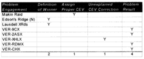
Next: WWII Cases

Validating A Combat Model (Part V)

[The article below is reprinted from April 1997 edition of The International TNDM Newsletter.]

The First Test of the TNDM Battalion-Level Validations: Predicting the Winners
by Christopher A. Lawrence

Part II

CONCLUSIONS:

WWI (12 cases):

For the WWI battles, the nature of the prediction problems are summarized as:

CONCLUSION: In the case of the WWI runs, five of the problem engagements were due to confusion of defining a winner or a clear CEV existing for a side that should have been predictable. Seven out of the 23 runs have some problems, with three problems resolving themselves by assigning a CEV value to a side that may not have deserved it. One (Medeah Farm) was just off any way you look at it, and three suffered a problems because historically the defenders (Germans) suffered surprisingly low losses. Two had the battle outcome predicted correctly on the first run, and then had the outcome incorrectly predicted after a CEV was assigned.

With 5 to 7 clear failures (depending on how you count them), this leads one to conclude that the TNDM can be relied upon to predict the winner in a WWI battalion-level battle in about 70% of the cases.

WWII (8 cases):

For the WWII battles, the nature of the prediction problems are summarized as:

CONCLUSION: In the case of the WWII runs, three of the problem engagements were due to confusion of defining a winner or a clear CEV existing for a side that should have been predictable. Four out of the 23 runs suffered a problem because historically the defenders (Germans) suffered surprisingly low losses and one case just simply assigned a possible unjustifiable CEV. This led to the battle outcome being predicted correctly on the first run, then incorrectly predicted after CEV was assigned.

With 3 to 5 clear failures, one can conclude that the TNDM can be relied upon to predict the winner in a WWII battalion-level battle in about 80% of the cases.

Modern (8 cases):

For the post-WWll battles, the nature of the prediction problems are summarized as:

CONCLUSION: ln the case of the modem runs, only one result was a problem. In the other seven cases, when the force with superior training is given a reasonable CEV (usually around 2), then the correct outcome is achieved. With only one clear failure, one can conclude that the TNDM can be relied upon to predict the winner in a modern battalion-level battle in over 90% of the cases.

FINAL CONCLUSIONS: In this article, the predictive ability of the model was examined only for its ability to predict the winner/loser. We did not look at the accuracy of the casualty predictions or the accuracy of the rates of advance. That will be done in the next two articles. Nonetheless, we could not help but notice some trends.

First and foremost, while the model was expected to be a reasonably good predictor of WWII combat, it did even better for modem combat. It was noticeably weaker for WWI combat. In the case of the WWI data, all attrition figures were multiplied by 4 ahead of time because we knew that there would be a fit problem otherwise.

This would strongly imply that there were more significant changes to warfare between 1918 and 1939 than between 1939 and 1989.

Secondly, the model is a pretty good predictor of winner and loser in WWII and modern cases. Overall, the model predicted the winner in 68% of the cases on the first run and in 84% of the cases in the run incorporating CEV. While its predictive powers were not perfect, there were 13 cases where it just wasn’t getting a good result (17%). Over half of these were from WWI, only one from the modern period.

In some of these battles it was pretty obvious who was going to win. Therefore, the model needed to do a step better than 50% to be even considered. Historically, in 51 out of 76 cases (67%). the larger side in the battle was the winner. One could predict the winner/loser with a reasonable degree of success by just looking at that rule. But the percentage of the time the larger side won varied widely with the period. In WWI the larger side won 74% of the time. In WWII it was 87%. In the modern period it was a counter-intuitive 47% of the time, yet the model was best at selecting the winner in the modern period.

The model’s ability to predict WWI battles is still questionable. It obviously does a pretty good job with WWII battles and appears to be doing an excellent job in the modern period. We suspect that the difference in prediction rates between WWII and the modern period is caused by the selection of battles, not by any inherit ability of the model.

RECOMMENDED CHANGES: While it is too early to settle upon a model improvement program, just looking at the problems of winning and losing, and the ancillary data to that, leads me to three corrections:

  1. Adjust for times of less than 24 hours. Create a formula so that battles of six hours in length are not 1/4 the casualties of a 24-hour battle, but something greater than that (possibly the square root of time). This adjustment should affect both casualties and advance rates.
  2. Adjust advance rates for smaller unit: to account for the fact that smaller units move faster than larger units.
  3. Adjust for fanaticism to account for those armies that continue to fight after most people would have accepted the result, driving up casualties for both sides.

Next Part III: Case Studies

Validating A Combat Model (Part IV)

[The article below is reprinted from April 1997 edition of The International TNDM Newsletter.]

The First Test of the TNDM Battalion-Level Validations: Predicting the Winners
by Christopher A. Lawrence

Part I

In the basic concept of the TNDM battalion-level validation, we decided to collect data from battles from three periods: WWI, WWII, and post-WWII. We then made a TNDM run for each battle exactly as the battle was laid out, with both sides having the same CEV [Combat Effectiveness Value]. The results of that run indicated what the CEV should have been for the battle, and we then made a second run using that CEV. That was all we did. We wanted to make sure that there was no “tweaking” of the model for the validation, so we stuck rigidly to this procedure. We then evaluated each run for its fit in three areas:

  1. Predicting the winner/loser
  2. Predicting the casualties
  3. Predicting the advance rate

We did end up changing two engagements around. We had a similar situation with one WWII engagement (Tenaru River) and one modern period engagement (Bir Gifgafa), where the defender received reinforcements part-way through the battle and counterattacked. In both cases we decided to run them as two separate battles (adding two more battles to our database), with the conditions from the first engagement being the starting strength, plus the reinforcements, for the second engagement. Based on our previous experience with running Goose Green, for all the Falklands Island battles we counted the Milans and Carl Gustavs as infantry weapons. That is the only “tweaking” we did that affected the battle outcome in the model. We also put in a casualty multiplier of 4 for WWI engagements, but that is discussed in the article on casualties.

This is the analysis of the first test, predicting the winner/loser. Basically, if the attacker won historically, we assigned it a value of 1, a draw was 0, and a defender win was -1. In the TNDM results summary, it has a column called “winner” which records either an attacker win, a draw, or a defender win. We compared these two results. If they were the same, this is a “correct” result. If they are “off by one,” this means the model predicted an attacker win or loss, where the actual result was a draw, or the model predicted a draw, where the actual result was a win or loss. If they are “off by two” then the model simply missed and predicted the wrong winner.

The results are (the envelope please….):

It is hard to determine a good predictability from a bad one. Obviously, the initial WWI prediction of 57% right is not very good, while the Modern second run result of 97% is quite good. What l would really like to do is compare these outputs to some other model (like TACWAR) to see if they get a closer fit. I have reason to believe that they will not do better.

Most cases in which the model was “off by 1″ were easily correctable by accounting for the different personnel capabilities of the army. Therefore, just to look where the model really failed. let‘s just look at where it simply got the wrong winner:

The TNDM is not designed or tested for WWI battles. It is basically designed to predict combat between 1939 and the present. The total percentages without the WWI data in it are:

Overall, based upon this data I would be willing to claim that the model can predict the correct winner 75% of the time without accounting for human factors and 90% of the time if it does.

CEVs: Quite simply a user of the TNDM must develop a CEV to get a good prediction. In this particular case, the CEVs were developed from the first run. This means that in the second run, the numbers have been juggled (by changing the CEV) to get a better result. This would make this effort meaningless if the CEVs were not fairly consistent over several engagements for one side versus its other side. Therefore, they are listed below in broad groupings so that the reader can determine if the CEVs appear to be basically valid or are simply being used as a “tweak.”

Now, let’s look where it went wrong. The following battles were not predicted correctly:

There are 19 night engagements in the data base, five from WWI, three from WWII, and 11 modern. We looked at whether the miss prediction was clustered among night engagements and that did not seem to be the case. Unable to find a pattern, we examined each engagement to see what the problem was. See the attachments at the end of this article for details.

We did obtain CEVs that showed some consistency. These are shown below. The Marines in World War l record the following CEVs in these WWI battles:

Compare those figures to the performance of the US Army:

In the above two and in all following cases, the italicized battles are the ones with which we had prediction problems.

For comparison purposes, the CEVs were recorded in the battles in World War II between the US and Japan:

For comparison purposes, the following CEVs were recorded in Operation Veritable:

These are the other engagements versus Germans for which CEVs were recorded:

For comparison purposes, the following CEVs were recorded in the post-WWII battles between Vietnamese forces and their opponents:

Note that the Americans have an average CEV advantage of 1 .6 over the NVA (only three cases) while having a 1.8 advantage over the VC (6 cases).

For comparison purposes, the following CEVs were recorded in the battles between the British and Argentine’s:

Next: Part II: Conclusions

Validating A Combat Model (Part III)

[The article below is reprinted from April 1997 edition of The International TNDM Newsletter.]

Numerical Adjustment of CEV Results: Averages and Means
by Christopher A. Lawrence and David L. Bongard

As part of the battalion-level validation effort, we made two runs with the model for each test case—one without CEV [Combat Effectiveness Value] incorporated and one with the CEV incorporated. The printout of a TNDM [Tactical Numerical Deterministic Model] run has three CEV figures for each side: CEVt CEVl and CEVad. CEVt shows the CEV as calculated on the basis of battlefield results as a ratio of the performance of side a versus side b. It measures performance based upon three factors: mission accomplishment, advance, and casualty effectiveness. CEVt is calculated according to the following formula:

P′ = Refined Combat Power Ratio (sum of the modified OLls). The ′ in P′ indicates that this ratio has been “refined” (modified) by two behavioral values already: the factor for Surprise and the Set Piece Factor.

CEVd = 1/CEVa (the reciprocal)

In effect the formula is relative results multiplied by the modified combat power ratio. This is basically the formulation that was used for the QJM [Quantified Judgement Model].

In the TNDM Manual, there is an alternate CEV method based upon comparative effective lethality. This methodology has the advantage that the user doesn’t have to evaluate mission accomplishment on a ten point scale. The CEVI calculated according to the following formula:

In effect, CEVt is a measurement of the difference in results predicted by the model from actual historical results based upon assessment for three different factors (mission success, advance rates, and casualties), while CEVl is a measurement of the difference in predicted casualties from actual casualties. The CEVt and the CEVl of the defender is the reciprocal of the one for the attacker.

Now the problem comes in when one creates the CEVad, which is the average of the two CEVs above. l simply do not know why it was decided to create an alternate CEV calculation from the old QJM method, and then average the two, but this is what is currently being done in the model. This averaging results in a revised CEV for the attacker and for the defender that are not reciprocals of each other, unless the CEVt and the CEVl were the same. We even have some cases where both sides had a CEVad of greater than one. Also, by averaging the two, we have heavily weighted casualty effectiveness relative to mission effectiveness and mission accomplishment.

What was done in these cases (again based more on TDI tradition or habit, and not on any specific rule) was:

(1.) If CEVad are reciprocals, then use as is.

(2.) If one CEV is greater than one while the other is less than 1,  then add the higher CEV to the value of the reciprocal of the lower CEV (1/x) and divide by two. This result is the CEV for the superior force, and its reciprocal is the CEV for the inferior force.

(3.) If both CEVs are above zero, then we divide the larger CEVad value by the smaller, and use its result as the superior force’s CEV.

In the case of (3.) above, this methodology usually results in a slightly higher CEV for the attacker side than if we used the average of the reciprocal (usually 0.1 or 0.2 higher). While the mathematical and logical consistency of the procedure bothered me, the logic for the different procedure in (3.) was that the model was clearly having a problem with predicting the engagement to start with, but that in most cases when this happened before (meaning before the validation), a higher CEV usually produced a better fit than a lower one. As this is what was done before. I accepted it as is, especially if one looks at the example of Mediah Farm. If one averages the reciprocal with the US’s CEV of 8.065, one would get a CEV of 4.13. By the methodology in (3.), one comes up with a more reasonable US CEV of 1.58.

The interesting aspect is that the TNDM rules manual explains how CEVt, CEVl and CEVad are calculated, but never is it explained which CEVad (attacker or defender) should be used. This is the first explanation of this process, and was based upon the “traditions” used at TDI. There is a strong argument to merge the two CEVs into one formulation. I am open to another methodology for calculating CEV. I am not satisfied with how CEV is calculated in the TNDM and intend to look into this further. Expect another article on this subject in the next issue.

Validating A Combat Model (Part II)

[The article below is reprinted from October 1996 edition of The International TNDM Newsletter.]

Validation of the TNDM at Battalion Level
by Christopher A. Lawrence

The original QJM (Quantified Judgement Model) was created and validated using primarily division-level engagements from WWII and the 1967 and 1973 Mid-East Wars. For a number of reasons, we are now using the TNDM (Tactical Numerical Deterministic Model) for analyzing lower-level engagements. We expect, with the changed environment in the world, this trend to continue.

The model, while designed to handle battalion-level engagements, was never validated for those size engagements. There were only 16 engagements in the original QJM Database with less than 5,000 people on one side, and only one with less than 2,000 people on a side. The sixteen smallest engagements are:

While it is not unusual in the operations research community to use unvalidated models of combat, it is a very poor practice. As TDI is starting to use this model for battalion-level engagements, it is time it was formally validated for that use. A model that is validated at one level of combat is not validated to represent sizes, types and forms of combat to which it has not been tested. TDI is undertaking a battalion-level validation effort for the TNDM. We intend to publish the material used and the results of the validation in the International TNDM Newsletter. As part of this battalion-level validation we will also be looking at a number of company-level engagements. Right now, my intention is to simply just throw all the engagements into the same hopper and see what comes out.

By battalion-level, I mean any operation consisting of the equivalent of two or less reinforced battalions on one side. Three or more battalions imply a regiment or brigade—level operation. A battalion in combat can range widely in strength, but that usually does not have an authorized strength in excess of 900. Therefore, the upper limit for a battalion—level engagement is 2,000 people, while its lower limit can easily go below 500 people. Only one engagement in the original OJM Database fits that definition of a battalion-level engagement. HERO, DMSI, TND & Associates, and TDI (all companies founded by Trevor N. Dupuy) examined a number of small engagements over the years. HERO assembled 23 WWI engagements for the Land Warfare Database (LWDB), TDI has done 15 WWII small unit actions for the Suppression contract and Dave Bongard has assembled four others from that period for the Pacific, DMSI did 14 battalion-level engagements from Vietnam for a study on low intensity conflict 10 years ago, and Dave Bongard has been independently looking into the Falkland Islands War and other post-WWII sources to locate 10 more engagements, and we have three engagements that Trevor N. Dupuy did for South Africa. We added two other World War II engagements and the three smallest engagements from the list to the left (those marked with an asterisk). This gives us a list of 74 additional engagements that can be used to test the TNDM.

The smallest of these engagements is 220 people on both sides (100 vs I20), while the largest engagement on this list is 5,336 versus 3,270 or 8,679 vs 725. These 74 engagements consist of 23 engagements from WWI, 22 from WWII, and 29 post-1945 engagements. There are three engagements where both sides have over 3,000 men and 3 more where both sides are above 2,000 men. In the other 68 engagements, at least one side is below 2,000, while in 50 of the engagements, both sides are below 2,000.

This leaves the following force sizes to be tested:

These engagements have been “randomly” selected in the sense that the researchers grabbed whatever had been done and whatever else was conveniently available. It is not a proper random selection, in the sense that every war in this century was analyzed and a representative number of engagements was taken from each conflict. This is not practical, so we settle for less than perfect data selection.

Furthermore, as many of these conflicts are with countries that do not have open archives (and in many cases limited unit records) some of the opposing forces strength and losses had to be estimated. This is especially true with the Viet Nam engagements. It is hoped that the errors in estimation deviate equally on both sides of the norm, but there is no way of knowing that until countries like the People’s Republic of China and Vietnam open up their archives for free independent research.

TDI intends to continue to look for battalion-level and smaller engagements for analysis, and may add to this data base over time. If some of our readers have any other data assembled, we would be interested in seeing it. In the next issue we will publish the preliminary results of our validation.

Note that in the above table, for World War II, German, Japanese, and Axis forces are listed in italics, while US, British, and Allied forces are listed in regular typeface, Also, in the VERITABLE engagements, the 5/7th Gordons’ action continues the assault of the 7th Black Watch, and that the 9th Cameronians assumed the attack begun by the 2d Gordon Highlanders.

Tu-Vu is described in some detail in Fall’s Street Without Joy (pp. 51-53). The remaining Indochina/SE Asia engagements listed here are drawn from a QJM-based analysis of low-intensity operations (HERO Report 124, Feb 1988).

The coding for source and validation status, on the extreme right of each engagement line in the D Cas column, is as follows:

  • n indicates an engagement which has not been employed for validation, but for which good data exists for both sides (35 total).
  • Q indicates an engagement which was part of the original QJM database (3 total).
  • Q+ indicates an engagement which was analyzed as part of the QJM low-intensity combat study in 1988 (14 total).
  • T indicates an engagement analyzed with the TNDM (20 total).

Validating A Combat Model

The question of validating combat models—“To confirm or prove that the output or outputs of a model are consistent with the real-world functioning or operation of the process, procedure, or activity which the model is intended to represent or replicate”—as Trevor Dupuy put it, has taken up a lot of space on the TDI blog this year. What this discussion did not address is what an effort to validate a combat model actually looks like. This will be the first in a series of posts that will do exactly that.

Under the guidance of Christopher A. Lawrence, TDI undertook a battalion-level validation of Dupuy’s Tactical Numerical Deterministic Model (TNDM) in late 1996. This effort tested the model against 76 engagements from World War I, World War II, and the post-1945 world including Vietnam, the Arab-Israeli Wars, the Falklands War, Angola, Nicaragua, etc. It was probably one of the more independent and better-documented validations of a casualty estimation methodology that has ever been conducted to date, in that:

  • The data was independently assembled (assembled for other purposes before the validation) by a number of different historians.
  • There were no calibration runs or adjustments made to the model before the test.
  • The data included a wide range of material from different conflicts and times (from 1918 to 1983).
  • The validation runs were conducted independently (Susan Rich conducted the validation runs, while Christopher A. Lawrence evaluated them).
  • The results of the validation were fully published.
  • The people conducting the validation were independent, in the sense that:

a) there was no contract, management, or agency requesting the validation;
b) none of the validators had previously been involved in designing the model, and had only very limited experience in using it; and
c) the original model designer was not able to oversee or influence the validation. (Dupuy passed away in July 1995 and the validation was conducted in 1996 and 1997.)

The validation was not truly independent, as the model tested was a commercial product of TDI, and the person conducting the test was an employee of the Institute. On the other hand, this was an independent effort in the sense that the effort was employee-initiated and not requested or reviewed by the management of the Institute.

Descriptions and outcomes of this validation effort were first reported in The International TNDM Newsletter. Chris Lawrence also addressed validation of the TNDM in Chapter 19 of War by Numbers (2017).

Counting Holes in Tanks in Tunisia

M4A1 Sherman destroyed in combat in Tunisia, 1943.

[NOTE: This piece was originally posted on 23 August 2016]

A few years ago, I came across a student battle analysis exercise prepared by the U.S. Army Combat Studies Institute on the Battle of Kasserine Pass in Tunisia in February 1943. At the time, I noted the diagram below (click for larger version), which showed the locations of U.S. tanks knocked out during a counterattack conducted by Combat Command C (CCC) of the U.S. 1st Armored Division against elements of the German 10th and 21st Panzer Divisions near the village of Sidi Bou Zid on 15 February 1943. Without reconnaissance and in the teeth of enemy air superiority, the inexperienced CCC attacked directly into a classic German tank ambush. CCC’s drive on Sidi Bou Zid was halted by a screen of German anti-tank guns, while elements of the two panzer divisions attacked the Americans on both flanks. By the time CCC withdrew several hours later, it had lost 46 of 52 M4 Sherman medium tanks, along with 15 officers and 298 men killed, captured, or missing.

Sidi Bou Zid00During a recent conversation with my colleague, Chris Lawrence, I recalled the diagram and became curious where it had originated. It identified the location of each destroyed tank, which company it belonged to, and what type of enemy weapon apparently destroyed it; significant battlefield features; and the general locations and movements of the enemy forces. What it revealed was significant. None of CCC’s M4 tanks were disabled or destroyed by a penetration of their frontal armor. Only one was hit by a German 88mm round from either the anti-tank guns or from the handful of available Panzer Mk. VI Tigers. All of the rest were hit with 50mm rounds from Panzer Mk. IIIs, which constituted most of the German force, or by 75mm rounds from Mk. IV’s. The Americans were not defeated by better German tanks. The M4 was superior to the Mk. III and equal to the Mk. IV; the dreaded 88mm anti-tank guns and Tiger tanks played little role in the destruction. The Americans had succumbed to superior German tactics and their own errors.

Counting dead tanks and analyzing their cause of death would have been an undertaking conducted by military operations researchers, at least in the early days of the profession. As Chris pointed out however, the Kasserine battle took place before the inception of operations research in the U.S. Army.

After a bit of digging online, I still have not been able to establish paternity of the diagram, but I think it was created as part of a battlefield survey conducted by the headquarters staff of either the U.S. 1st Armored Division, or one of its subordinate combat commands. The only reference I can find for it is as part of a historical report compiled by Brigadier General Paul Robinett, submitted to support the preparation of Northwest Africa: Seizing the Initiative in the West by George F. Howe, the U.S. Army Center of Military History’s (CMH) official history volume on U.S. Army operations in North Africa, published in 1956. Robinett was the commander of Combat Command B, U.S. 1st Armored Division during the Battle of Kasserine Pass, but did not participate in the engagement at Sidi Bou Zid. His report is excerpted in a set of readings (pp. 103-120) provided as background material for a Kasserine Pass staff ride prepared by CMH. (Curiously, the account of the 15 February engagement at Sidi Bou Zid in Northwest Africa [pp. 419-422] does not reference Robinett’s study.)

Robinett’s report appeared to include an annotated copy of a topographical map labeled “approximate location of destroyed U.S. tanks (as surveyed three weeks later).” This suggests that the battlefield was surveyed in late March 1943, after U.S. forces had defeated the Germans and regained control of the area.

Sidi Bou Zid02The report also included a version of the schematic diagram later reproduced by CMH. The notes on the map seem to indicate that the survey was the work of staff officers, perhaps at Robinett’s direction, possibly as part of an after-action report.

Sidi Bou Zid03If anyone knows more about the origins of this bit of battlefield archaeology, I would love to know more about it. As far as I know, this assessment was unique, at least in the U.S. Army in World War II.

Trevor Dupuy’s Definitions of Lethality

Two U.S. Marines with a M1919A4 machine gun on Roi-Namur Island in the Marshall Islands during World War II. [Wikimedia]

It appears that discussion of the meaning of lethality, as related to the use of the term in the 2018 U.S. National Defense Strategy document, has sparked up again. It was kicked off by an interesting piece by Olivia Gerard in The Strategy Bridge last autumn, “Lethality: An Inquiry.

Gerard credited Trevor Dupuy and his colleagues at the Historical Evaluation Research Organization (HERO) with codifying “the military appropriation of the concept” of lethality, which was defined as: “the inherent capability of a given weapon to kill personnel or make materiel ineffective in a given period, where capability includes the factors of weapon range, rate of fire, accuracy, radius of effects, and battlefield mobility.”

It is gratifying for Gerard to attribute this to Dupuy and HERO, but some clarification is needed. The definition she quoted was, in fact, one provided to HERO for the purposes of a study sponsored by the Advanced Tactics Project (AVTAC) of the U.S. Army Combat Developments Command. The 1964 study report, Historical Trends Related to Weapon Lethality, provided the starting point for Dupuy’s subsequent theorizing about combat.

In his own works, Dupuy used a simpler definition of lethality:

He also used the terms lethality and firepower interchangeably in his writings. The wording of the original 1964 AVTAC definition tracks closely with the lethality scoring methodology Dupuy and his HERO colleagues developed for the study, known as the Theoretical Lethality Index/Operational Lethality Index (TLI/OLI). The original purpose of this construct was to permit some measurement of lethality by which weapons could be compared to each other (TLI), and to each other through history (OLI). It worked well enough that he incorporated it into his combat models, the Quantified Judgement Model (QJM) and Tactical Numerical Deterministic Model (TNDM).

Dupuy’s Verities: The Complexities of Combat

“The Battle of Leipzig, 16-19 October 1813” by A.I. Zauerweid (1783-1844) [Wikimedia]
The thirteenth and last of Trevor Dupuy’s Timeless Verities of Combat is:

Combat is too complex to be described in a single, simple aphorism.

From Understanding War (1987):

This is amply demonstrated by the preceding [verities]. All writers on military affairs (including this one) need periodically to remind themselves of this. In military analysis it is often necessary to focus on some particular aspect of combat. However, the results of such closely focused analyses must the be evaluated in the context of the brutal, multifarious, overlapping realities of war.

Trevor Dupuy was sometimes accused of attempting to reduce war to a mathematical equation. A casual reading of his writings might give that impression, but anyone who honestly engages with his ideas quickly finds this to be an erroneous conclusion. Yet, Dupuy believed the temptation to simplify and abstract combat and warfare to be common enough that he he embedded a warning against doing so into his basic theory on the subject. He firmly believed that human behavior comprises the most important aspect of combat, yet it is all too easy to miss the human experience of war figuring who lost or won and why, and counts of weapons, people, and casualties. As a military historian, he was keenly aware that the human stories behind the numbers—however imperfectly recorded and told—tell us more about the reality of war than mere numbers on their own ever will.

Dupuy’s Verities: The Inefficiency of Combat

The “Mud March” of the Union Army of the Potomac, January 1863.

The twelfth of Trevor Dupuy’s Timeless Verities of Combat is:

Combat activities are always slower, less productive, and less efficient than anticipated.

From Understanding War (1987):

This is the phenomenon that Clausewitz called “friction in war.” Friction is largely due to the disruptive, suppressive, and dispersal effects of firepower upon an aggregation of people. This pace of actual combat operations will be much slower than the progress of field tests and training exercises, even highly realistic ones. Tests and exercises are not truly realistic portrayals of combat, because they lack the element of fear in a lethal environment, present only in real combat. Allowances must be made in planning and execution for the effects of friction, including mistakes, breakdowns, and confusion.

While Clausewitz asserted that the effects of friction on the battlefield could not be measured because they were largely due to chance, Dupuy believed that its influence could, in fact, be gauged and quantified. He identified at least two distinct combat phenomena he thought reflected measurable effects of friction: the differences in casualty rates between large and small sized forces, and diminishing returns from adding extra combat power beyond a certain point in battle. He also believed much more research would be necessary to fully understand and account for this.

Dupuy was skeptical of the accuracy of combat models that failed to account for this interaction between operational and human factors on the battlefield. He was particularly doubtful about approaches that started by calculating the outcomes of combat between individual small-sized units or weapons platforms based on the Lanchester equations or “physics-based” estimates, then used these as inputs for brigade and division-level-battles, the results of which in turn were used as the basis for determining the consequences of theater-level campaigns. He thought that such models, known as “bottom up,” hierarchical, or aggregated concepts (and the prevailing approach to campaign combat modeling in the U.S.), would be incapable of accurately capturing and simulating the effects of friction.