Tag combat

Comparing the RAND Version of the 3:1 Rule to Real-World Data

Chuliengcheng. In a glorious death eternal life. (Battle of Yalu River, 1904) [Wikimedia Commons]

[The article below is reprinted from the Winter 2010 edition of The International TNDM Newsletter.]

Comparing the RAND Version of the 3:1 Rule to Real-World Data
Christopher A. Lawrence

For this test, The Dupuy Institute took advan­tage of two of its existing databases for the DuWar suite of databases. The first is the Battles Database (BaDB), which covers 243 battles from 1600 to 1900. The sec­ond is the Division-level Engagement Database (DLEDB), which covers 675 division-level engagements from 1904 to 1991.

The first was chosen to provide a historical con­text for the 3:1 rule of thumb. The second was chosen so as to examine how this rule applies to modern com­bat data.

We decided that this should be tested to the RAND version of the 3:1 rule as documented by RAND in 1992 and used in JICM [Joint Integrated Contingency Model] (with SFS [Situational Force Scoring]) and other mod­els. This rule, as presented by RAND, states: “[T]he famous ‘3:1 rule,’ according to which the attacker and defender suffer equal fractional loss rates at a 3:1 force ratio if the battle is in mixed terrain and the defender enjoys ‘prepared’ defenses…”

Therefore, we selected out all those engage­ments from these two databases that ranged from force ratios of 2.5 to 1 to 3.5 to 1 (inclusive). It was then a simple matter to map those to a chart that looked at attackers losses compared to defender losses. In the case of the pre-1904 cases, even with a large database (243 cases), there were only 12 cases of combat in that range, hardly statistically significant. That was because most of the combat was at odds ratios in the range of .50-to-1 to 2.00-to-one.

The count of number of engagements by odds in the pre-1904 cases:

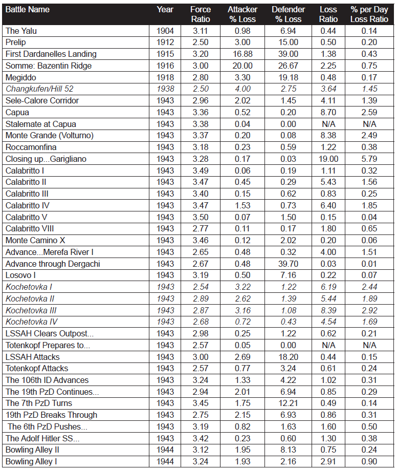
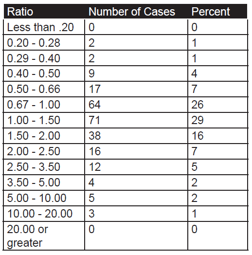
As the database is one of battles, then usually these are only joined at reasonably favorable odds, as shown by the fact that 88 percent of the battles occur between 0.40 and 2.50 to 1 odds. The twelve pre-1904 cases in the range of 2.50 to 3.50 are shown in Table 1.

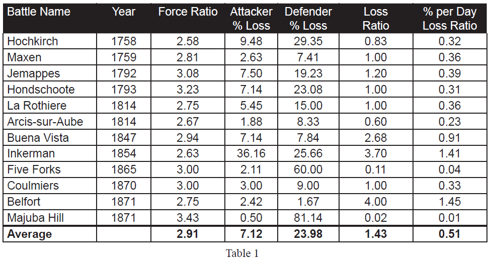
If the RAND version of the 3:1 rule was valid, one would expect that the “Percent per Day Loss Ratio” (the last column) would hover around 1.00, as this is the ratio of attacker percent loss rate to the defender per­cent loss rate. As it is, 9 of the 12 data points are notice­ably below 1 (below 0.40 or a 1 to 2.50 exchange rate). This leaves only three cases (25%) with an exchange rate that would support such a “rule.”

If we look at the simple ratio of actual losses (vice percent losses), then the numbers comes much closer to parity, but this is not the RAND interpreta­tion of the 3:1 rule. Six of the twelve numbers “hover” around an even exchange ratio, with six other sets of data being widely off that central point. “Hover” for the rest of this discussion means that the exchange ratio ranges from 0.50-to-1 to 2.00-to 1.

Still, this is early modern linear combat, and is not always representative of modern war. Instead, we will examine 634 cases in the Division-level Database (which consists of 675 cases) where we have worked out the force ratios. While this database covers from 1904 to 1991, most of the cases are from WWII (1939- 1945). Just to compare:

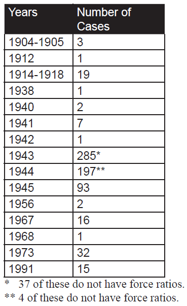
As such, 87% of the cases are from WWII data and 10% of the cases are from post-WWII data. The engagements without force ratios are those that we are still working on as The Dupuy Institute is always ex­panding the DLEDB as a matter of routine. The specific cases, where the force ratios are between 2.50 and 3.50 to 1 (inclusive) are shown in Table 2:

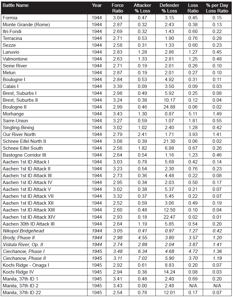
This is a total of 98 engagements at force ratios of 2.50 to 3.50 to 1. It is 15 percent of the 634 engage­ments for which we had force ratios. With this fairly significant representation of the overall population, we are still getting no indication that the 3:1 rule, as RAND postulates it applies to casualties, does indeed fit the data at all. Of the 98 engagements, only 19 of them demonstrate a percent per day loss ratio (casualty exchange ratio) between 0.50-to-1 and 2-to-1. This is only 19 percent of the engagements at roughly 3:1 force ratio. There were 72 percent (71 cases) of those engage­ments at lower figures (below 0.50-to-1) and only 8 percent (cases) are at a higher exchange ratio. The data clearly was not clustered around the area from 0.50-to- 1 to 2-to-1 range, but was well to the left (lower) of it.

Looking just at straight exchange ratios, we do get a better fit, with 31 percent (30 cases) of the figure ranging between 0.50 to 1 and 2 to 1. Still, this fig­ure exchange might not be the norm with 45 percent (44 cases) lower and 24 percent (24 cases) higher. By definition, this fit is 1/3rd the losses for the attacker as postulated in the RAND version of the 3:1 rule. This is effectively an order of magnitude difference, and it clearly does not represent the norm or the center case.

The percent per day loss exchange ratio ranges from 0.00 to 5.71. The data tends to be clustered at the lower values, so the high values are very much outliers. The highest percent exchange ratio is 5.71, the second highest is 4.41, the third highest is 2.92. At the other end of the spectrum, there are four cases where no losses were suffered by one side and seven where the exchange ratio was .01 or less. Ignoring the “N/A” (no losses suffered by one side) and the two high “outliers (5.71 and 4.41), leaves a range of values from 0.00 to 2.92 across 92 cases. With an even dis­tribution across that range, one would expect that 51 percent of them would be in the range of 0.50-to-1 and 2.00-to-1. With only 19 percent of the cases being in that range, one is left to conclude that there is no clear correlation here. In fact, it clearly is the opposite effect, which is that there is a negative relationship. Not only is the RAND construct unsupported, it is clearly and soundly contradicted with this data. Furthermore, the RAND construct is theoretically a worse predictor of casualty rates than if one randomly selected a value for the percentile exchange rates between the range of 0 and 2.92. We do believe this data is appropriate and ac­curate for such a test.

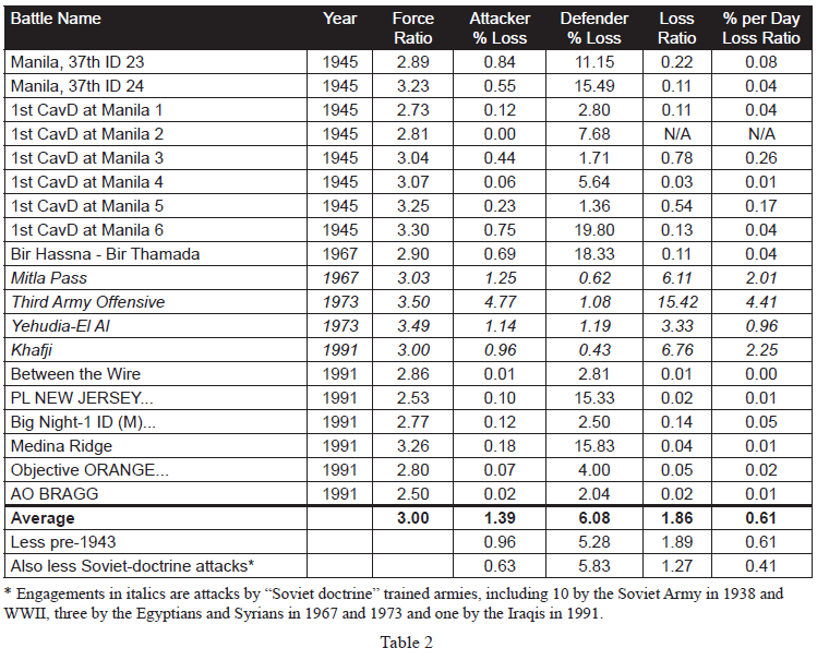
As there are only 19 cases of 3:1 attacks fall­ing in the even percentile exchange rate range, then we should probably look at these cases for a moment:

One will note, in these 19 cases, that the aver­age attacker casualties are way out of line with the av­erage for the entire data set (3.20 versus 1.39 or 3.20 versus 0.63 with pre-1943 and Soviet-doctrine attack­ers removed). The reverse is the case for the defenders (3.12 versus 6.08 or 3.12 versus 5.83 with pre-1943 and Soviet-doctrine attackers removed). Of course, of the 19 cases, 2 are pre-1943 cases and 7 are cases of Soviet-doctrine attackers (in fact, 8 of the 14 cases of the So­viet-doctrine attackers are in this selection of 19 cases). This leaves 10 other cases from the Mediterranean and ETO (Northwest Europe 1944). These are clearly the unusual cases, outliers, etc. While the RAND 3:1 rule may be applicable for the Soviet-doctrine offensives (as it applies to 8 of the 14 such cases we have), it does not appear to be applicable to anything else. By the same token, it also does not appear to apply to virtually any cases of post-WWII combat. This all strongly argues that not only is the RAND construct not proven, but it is indeed clearly not correct.

The fact that this construct also appears in So­viet literature, but nowhere else in US literature, indi­cates that this is indeed where the rule was drawn from. One must consider the original scenarios run for the RSAC [RAND Strategy Assessment Center] wargame were “Fulda Gap” and Korean War scenarios. As such, they were regularly conducting bat­tles with Soviet attackers versus Allied defenders. It would appear that the 3:1 rule that they used more closely reflected the experiences of the Soviet attackers in WWII than anything else. Therefore, it may have been a fine representation for those scenarios as long as there was no US counterattacking or US offensives (and assuming that the Soviet Army of the 1980s performed at the same level as in did in the 1940s).

There was a clear relative performance difference between the Soviet Army and the German Army in World War II (see our Capture Rate Study Phase I & II and Measuring Human Factors in Combat for a detailed analysis of this).[1] It was roughly in the order of a 3-to-1-casualty exchange ratio. Therefore, it is not surprising that Soviet writers would create analytical tables based upon an equal percentage exchange of losses when attacking at 3:1. What is surprising, is that such a table would be used in the US to represent US forces now. This is clearly not a correct application.

Therefore, RAND’s SFS, as currently con­structed, is calibrated to, and should only be used to represent, a Soviet-doctrine attack on first world forces where the Soviet-style attacker is clearly not properly trained and where the degree of performance difference is similar to that between the Germans and Soviets in 1942-44. It should not be used for US counterattacks, US attacks, or for any forces of roughly comparable ability (regardless of whether Soviet-style doctrine or not). Furthermore, it should not be used for US attacks against forces of inferior training, motivation and co­hesiveness. If it is, then any such tables should be ex­pected to produce incorrect results, with attacker losses being far too high relative to the defender. In effect, the tables unrealistically penalize the attacker.

As JICM with SFS is now being used for a wide variety of scenarios, then it should not be used at all until this fundamental error is corrected, even if that use is only for training. With combat tables keyed to a result that is clearly off by an order of magnitude, then the danger of negative training is high.

NOTES

[1] Capture Rate Study Phases I and II Final Report (The Dupuy Institute, March 6, 2000) (2 Vols.) and Measuring Human Fac­tors in Combat—Part of the Enemy Prisoner of War Capture Rate Study (The Dupuy Institute, August 31, 2000). Both of these reports are available through our web site.

Aerial Combined Arms

In a previous post, I quoted Jules Hurst’s comparison between the medieval knights of old and modern day fighter pilots. His point was that the future of aerial combat will feature more combined arms. This I agree with; the degree of specialization that will be seen in the future will increase, although our ability to predict what this will be is uncertain. Hurst’s second point, that today’s aerial combat is akin to jousting and jovial knights looking to independently take down foes, I do not agree with at all.

Last night, I watched the History Channel documentary “Dogfights of Desert Storm,” a wonderful summary of several selected dogfights from the first Gulf War (1991, US and coalition vs Iraq), which included:

1. A furball between an unarmed EF-111 and a Mirage F1. Eventually, an F-15C came to the rescue, but the EF-111 crew was apparently awarded the Distinguished Flying Cross for its actions that day. Ultimately, the F1 hit the ground, and the F-15C got the credit.

2. A complex dogfight between a flight of two F-15Cs against 2 Mig-25s and 2 Mig-29s. This was a hairy affair, with lots of maneuver. The MiG-25s were able to decoy many heat-seeking AIM-9’s, so the AIM-7 radar guided missiles needed to be used to shoot them down.

[As previously reported, an F/A-18F had problems trying to down a Syrian Su-22 Fitter with an AIM-9 missile due to the effectiveness of Russian-made flares and had to resort to an AIM-120 radar-guided missile. Also a strategy from Soviet days, the preference to carry more than one type of seeker types seems to be quite good advice. The U.S. Air Force (USAF) has traditionally adhered to the concept of a beyond visual range (BVR) medium range, radar guided missile, the AIM-7 and the AIM-120 successor. This coupled with the short range AIM-9 infrared missile. The gap that this leaves is the long range, infrared guided missile.]

3. A well-run dogfight pitting a flight of four F-15Cs vs. a flight of four F-1s. Of the F-1s, one turned back to base, either for fear, prudence, or mechanical difficulty, it is difficult to say. The three other F-1s were all downed by AIM-7 missiles, fired at beyond visual range. What was noted about this engagement was the patience of the USAF flight leader, who did not immediately lock-on to the F-1s, in order to avoid triggering their radar warning receivers (RWR), and giving up the element of surprise by notifying them of the impending attack.

The statistic given was that 60% of the aerial victories in the entire conflict were from BVR.

The coalition’s triumph was an emphatic boost for current air war strategy. Multiple aircraft with specific roles working on concert to achieve victory. Air war in 1990, as it is today, is a team sport.” Multiple weapons disrupted the Iraqi capability to deal with it. It was information overload. They could not deal with the multiple successive strikes, and the fact that their radars went offline, and their command and control was shut down … jamming … deception – it was like having essentially a ‘war nervous breakdown’. (emphasis added).

Larry Pitts, a USAF F-15C Eagle pilot (retired), said

aerial victory against an enemy airplane was a career highlight for me. It’s something that I’ll never be able to beat, but you know in my mind, I did what any fighter pilot would have done if any enemy fighter had been put in front of him. I relied on my training, I engaged the airplane, protected my wingman as he protected me, and came out of it alive.

One key element in all of the combat recounted by the USAF pilots was the presence of airborne early warning aircraft, at the time the E-3C Sentry. Indeed, this form of combined arms—which is effectively an augmentation of a fighter pilot’s sensors—has been around for a surprisingly long time.

  • In February 1944, the United States Navy (USN), under Project Cadillac, equipped a TBM Avenger torpedo bomber with an airborne radar, and the resulting TBM-3W entered service with the Airborne Early Warning (AEW) mission.
  • In June 1949, a joint program with the USN and USAF resulted in the EC-121 Warning Star, a conversion of a Lockheed L1094 Super Constellation airliner. This aircraft entered service to reinforce the Distant Early Warning (DEW) Line, across the Arctic in Canada and Alaska to detect and defend against Soviet Air Force bombers flying over the pole. This was also the plane that played the “AWACS” role in Vietnam.
  • In January 1964, the E-2 Hawkeye was introduced into service with the USN, which required a carrier-based AWACS platform.
  • In March 1977, the first E-3 Sentry was delivered to the USAF by Boeing.

Indeed, the chart below illustrates the wide variety of roles and platforms flown by the USAF, in their combined arms operations.

[Source: Command: Modern Air & Naval Operations]

In addition, the USAF just released its FY2019 budget, fresh from budget action in Congress. This had a few surprises, including the planned retirement of both the B-1B and the B-2A in favor of the upcoming B-21 Raider, and continuing to enhance and improve the B-52. This is a very old platform, having been introduced in 1955. This does match a shift in thinking by the USAF, from stating that all of the fourth generation aircraft (non-stealthy) are entirely obsolete, to one in which they continue to play a role, as a follow-up force, perhaps in role of a “distant archer” with stand-off weapons. I previously discussed the Talon Hate pod enabling network communications between the F-22 and F-15C systems.

More on this to come!

Spotted In The New Books Section Of The U.S. Naval Academy Library…

Christopher A. Lawrence, War by Numbers: Understanding Conventional Combat (Lincoln, NE: Potomac Books, 2017) 390 pages, $39.95

War by Numbers assesses the nature of conventional warfare through the analysis of historical combat. Christopher A. Lawrence (President and Executive Director of The Dupuy Institute) establishes what we know about conventional combat and why we know it. By demonstrating the impact a variety of factors have on combat he moves such analysis beyond the work of Carl von Clausewitz and into modern data and interpretation.

Using vast data sets, Lawrence examines force ratios, the human factor in case studies from World War II and beyond, the combat value of superior situational awareness, and the effects of dispersion, among other elements. Lawrence challenges existing interpretations of conventional warfare and shows how such combat should be conducted in the future, simultaneously broadening our understanding of what it means to fight wars by the numbers.

The book is available in paperback directly from Potomac Books and in paperback and Kindle from Amazon.

Russian Army Experiments With Using Tanks For Indirect Fire

Russian Army T-90S main battle tanks. [Ministry of Defense of the Russian Federation]

Finnish freelance writer and military blogger Petri Mäkelä spotted an interesting announcement from the Ministry of Defense of the Russian Federation: the Combined-Arms Army of the Western Military District is currently testing the use of main battle tanks for indirect fire at the Pogonovo test range in the Voronezh region.

According to Major General Timur Trubiyenko, First Deputy Commander of the Western Military District Combined-Arms Army, in the course of company exercises, 200 tankers will test a combination of platoon direct and indirect fire tactics against simulated armored, lightly armored, and concealed targets up to 12 kilometers away.

Per Mäkelä, the exercise will involve T-90S main battle tanks using their 2A46 125 mm/L48 smoothbore cannons. According to the Ministry of Defense, more than 1,000 Russian Army soldiers, employing over 100 weapons systems and special equipment items, will participate in the exercises between 19 and 22 February 2018.

Tanks have been used on occasion to deliver indirect fire in World War II and Korea, but it is not a commonly used modern tactic. The use of modern fire control systems, guided rounds, and drone spotters might offer the means to make this more useful.

Aerial Drone Tactics, 2025-2050

[Image: War On The Rocks.]

My previous post outlined the potential advantages and limitations of current and future drone technology. The real utility of drones in future warfare may lie in a tactic that is both quite old and new, swarming. “‘This [drone swarm concept] goes all the way back to the tactics of Attila the Hun,’ says Randall Steeb, senior engineer at the Rand Corporation in the US. ‘A light attack force that can defeat more powerful and sophisticated opponents. They come out of nowhere, attack from all sides and then disappear, over and over.'”

In order to be effective, Mr. Steeb’s concept would require drones to be able to speed away from their adversary, or be able to hide. The Huns are described “as preferring to defeat their enemies by deceit, surprise attacks, and cutting off supplies. The Huns brought large numbers of horses to use as replacements and to give the impression of a larger army on campaign.” Also, prior to problems caused to the Roman Empire by the Huns under Attila (~400 CE), another group of people, the Scythians, used similar tactics much earlier, as mentioned by Herodotus, (~800 BCE). “With great mobility, the Scythians could absorb the attacks of more cumbersome foot soldiers and cavalry, just retreating into the steppes. Such tactics wore down their enemies, making them easier to defeat.” These tactics were also used by the Parthians, resulted in the Roman defeat under Crassis at the Battle of Carrahe, 53 BCE. Clearly, maneuver is as old as warfare itself.

Indeed, others have their own ancient analogies.

Today, fighter pilots approach warfare like a questing medieval knight. They search for opponents with similar capabilities and defeat them by using technologically superior equipment or better application of individual tactics and techniques. For decades, leading air forces nurtured this dynamic by developing expensive, manned air superiority fighters. This will all soon change. Advances in unmanned combat aerial vehicles (UCAVs) will turn fighter pilots from noble combatants to small-unit leaders and drive the development of new aerial combined arms tactics.

Drone Swarms: A Game Changer?

We can see that the new technologies come along, and they enable a new look at warfare, and often enable a new implementation of ancient tactics. There are some who claim that this changes the game, and indeed may change the fundamental nature of war.

Peter Singer, an expert on future warfare at the New America think-tank, is in no doubt. ‘What we have is a series of technologies that change the game. They’re not science fiction. They raise new questions. What’s possible? What’s proper?’ Mr. Singer is talking about artificial intelligence, machine learning, robotics and big-data analytics. Together they will produce systems and weapons with varying degrees of autonomy, from being able to work under human supervision to ‘thinking’ for themselves. The most decisive factor on the battlefield of the future may be the quality of each side’s algorithms. Combat may speed up so much that humans can no longer keep up. Frank Hoffman, a fellow of the National Defense University who coined the term ‘hybrid warfare’, believes that these new technologies have the potential not just to change the character of war but even possibly its supposedly immutable nature as a contest of wills. For the first time, the human factors that have defined success in war, ‘will, fear, decision-making and even the human spark of genius, may be less evident,’ he says.” (emphasis added).

Drones are highly capable, and with increasing autonomy, they themselves may be immune to fear. Technology has been progressing step by step to alter the character of war. Think of the Roman soldier and his personal experience in warfare up close vs. the modern sniper. They each have a different experience in warfare, and fear manifests itself in different ways. Unless we create and deploy full autonomous systems, with no human in or on the loop, there will be an opportunity for fear and confusion by the human mind to creep into martial matters. An indeed, with so much new technology, friction of some sort is almost assured.

I’m not alone in this assessment. Secretary of Defense James Mattis has said “You go all the way back to Thucydides who wrote the first history and it was of a war and he said it’s fear and honor and interest and those continue to this day. The fundamental nature of war is unchanging. War is a human social phenomenon.”

Swarming and Information Dominance

Indeed, the notion of the importance of information dominance plays upon one of the most important fundamental aspects of warfare: surprise. There are many synonyms for surprise, one of the most popular these days is situational awareness (SA). In a recent assessment of trends in air-to-air combat for the Center for Strategic and Budgetary Assessments (CSBA), Dr. John Stillion described the impact of SA.

Aerial combat over the past two decades, though relatively rare, continues to demonstrate the importance of superior SA. The building blocks, however, of superior SA, information acquisition and information denial, seem to be increasingly associated with sensors, signature reduction, and networks. Looking forward, these changes have greatly increased the proportion of BVR [Beyond Visual Range] engagements and likely reduced the utility of traditional fighter aircraft attributes, such as speed and maneuverability, in aerial combat. At the same time, they seem to have increased the importance of other attributes.

Stillion, famous for his RAND briefing on the F-35, proposes an interesting concept of operations for air-to-air combat, centered on larger aircraft with bigger sensor apertures, and subsonic UCAS fighters in the “front line.” He’s got a good video to illustrate how this concept would work against an adversary.

[I]t is important to acknowledge that all of the foregoing discussion is based on certain assumptions plus analysis of past trends, and the future of aerial combat might continue to belong to fast, agile aircraft. The alternative vision of future aerial combat presented in Chapter 5 relies heavily on robust LoS [Line of Sight] data links to enable widely distributed aircraft to efficiently share information and act in concert to achieve superior SA and combat effectiveness. Should the links be degraded or denied, the concept put forward here would be difficult or impossible to implement.

Therefore, in the near term, one of the most important capabilities to enable is a secure battle network. This will be required for remotely piloted and autonomous system alike, and this will be the foundation of information dominance – the acquisition of information for use by friendly forces, and the denial of information to an adversary.

Air Power and Drones, 2025-2050

[Credit: Financial Times]

In the recently issued 2018 National Defense Strategy, the United States acknowledged that “long-term strategic competitions with China and Russia are the principal priorities for the Department [of Defense], and require both increased and sustained investment, because of the magnitude of the threats they pose to U.S. security and prosperity today, and the potential for those threats to increase in the future.”

The strategy statement lists technologies that will be focused upon:

The drive to develop new technologies is relentless, expanding to more actors with lower barriers of entry, and moving at accelerating speed. New technologies include advanced computing, “big data” analytics, artificial intelligence, autonomy, robotics, directed energy, hypersonics, and biotechnology— the very technologies that ensure we will be able to fight and win the wars of the future… The Department will invest broadly in military application of autonomy, artificial intelligence, and machine learning, including rapid application of commercial breakthroughs, to gain competitive military advantages.” (emphasis added).

Autonomy, robotics, artificial intelligence and machine learning…these are all related to the concept of “drone swarms.” TDI has reported previously on the idea of drone swarms on land. There is indeed promise in many domains of warfare for such technology. In testimony to the Senate Armed Services Committee on the future of warfare, Mr Bryan Clark of the Center for Strategic and Budgetary Assessments argued that “America should apply new technologies to four main areas of warfare: undersea, strike, air and electromagnetic.”

Drones have certainly transformed the way that the U.S. wages war from the air. The Central Intelligence Agency (CIA) innovated, deployed and fired weapons from drones first against the Taliban in Afghanistan, less than one month after the 9/11 attacks against the U.S. homeland. Most drones today are airborne, partly because it is generally easier to navigate in the air than it is on the land, due to fewer obstacles and more uniform and predictable terrain. The same is largely true of the oceans, at least the blue water parts.

Aerial Drones and Artificial Intelligence

It is important to note that the drones in active use today by the U.S. military are actually remotely piloted Unmanned Aerial Vehicles (UAVs). With the ability to fire missiles since 2001, one could argue that these crossed the threshold into Unmanned Combat Aerial Vehicles (UCAVs), but nonetheless, they have a pilot—typically a U.S. Air Force (USAF) member, who would very much like to be flying an F-16, rather than sitting in a shipping container in the desert somewhere safe, piloting a UAV in a distant theater of war.

Given these morale challenges, work on autonomy is clearly underway. Let’s look at a forecast from The Economist, which follows the development of artificial intelligence (AI) in both the commercial and military realms.

A distinction needs to be made between “narrow” AI, which allows a machine to carry out a specific task much better than a human could, and “general” AI, which has far broader applications. Narrow AI is already in wide use for civilian tasks such as search and translation, spam filters, autonomous vehicles, high-frequency stock trading and chess-playing computers… General AI may still be at least 20 years off. A general AI machine should be able to carry out almost any intellectual task that a human is capable of.” (emphasis added)

Thus, it is reasonable to assume that the U.S. military (or others) will not field a fully automated drone, capable of prosecuting a battle without human assistance, until roughly 2038. This means that in the meantime, a human will be somewhere “in” or “on” the loop, making at least some of the decisions, especially those involving deadly force.

[Credit: The Economist]
Future Aerial Drone Roles and Missions

The CIA’s initial generation of UAVs was armed in an ad-hoc fashion; further innovation was spurred by the drive to seek out and destroy the 9/11 perpetrators. These early vehicles were designed for intelligence, reconnaissance, and surveillance (ISR) missions. In this role, drones have some big advantages over manned aircraft, including the ability to loiter for long periods. They are not quick, not very maneuverable, and as such are suited to operations in permissive airspace.

The development of UCAVs has allowed their integration into strike (air-to-ground) and air superiority (air-to-air) missions in contested airspace. UCAV strike missions could target and destroy land and sea nodes in command, control, communications, computers, intelligence, surveillance and reconnaissance (C4ISR) networks in an attempt to establish “information dominance.” They might also be targeted against assets like surface to air missiles and radars, part of an adversary anti-access/area denial (A2/AD) capability.

Given the sophistication of Russian and Chinese A2/AD networks and air forces, some focus should be placed upon developing more capable and advanced drones required to defeat these challenges. One example comes from Kratos, a drone maker, and reported on in Popular Science.

Concept art for Mako combat drone. Based on the existing BQM-167 aerial target, this drone can maneuver at forces that could kill a human pilot [Image courtesy of Kratos/Popular Science]

The Mako drone pictured above has much higher performance than some other visions of future drone swarms, which look more like paper airplanes. Given their size and numbers, they might be difficult to shoot down entirely, and this might be able to operate reasonably well within contested airspace. But, they’re not well suited for air-to-air combat, as they will not have the weapons or the speed necessary to engage with current manned aircraft in use with potential enemy air forces. Left unchecked, an adversary’s current fighters and bombers could easily avoid these types of drones and prosecute their own attacks on vital systems, installations and facilities.

The real utility of drones may lie in the unique tactic for which they are suited, swarming. More on that in my next post.

Attrition In Future Land Combat

Soldiers with Battery C, 1st Battalion, 82nd Field Artillery Regiment, 1st Brigade Combat Team, 1st Cavalry Division maneuver their Paladins through Hohenfels Training Area, Oct. 26. Photo Credit: Capt. John Farmer, 1st Brigade Combat Team, 1st Cav

[This post was originally published on June 9, 2017]

Last autumn, U.S. Army Chief of Staff General Mark Milley asserted that “we are on the cusp of a fundamental change in the character of warfare, and specifically ground warfare. It will be highly lethal, very highly lethal, unlike anything our Army has experienced, at least since World War II.” He made these comments while describing the Army’s evolving Multi-Domain Battle concept for waging future combat against peer or near-peer adversaries.

How lethal will combat on future battlefields be? Forecasting the future is, of course, an undertaking fraught with uncertainties. Milley’s comments undoubtedly reflect the Army’s best guesses about the likely impact of new weapons systems of greater lethality and accuracy, as well as improved capabilities for acquiring targets. Many observers have been closely watching the use of such weapons on the battlefield in the Ukraine. The spectacular success of the Zelenopillya rocket strike in 2014 was a convincing display of the lethality of long-range precision strike capabilities.

It is possible that ground combat attrition in the future between peer or near-peer combatants may be comparable to the U.S. experience in World War II (although there were considerable differences between the experiences of the various belligerents). Combat losses could be heavier. It certainly seems likely that they would be higher than those experienced by U.S. forces in recent counterinsurgency operations.

Unfortunately, the U.S. Defense Department has demonstrated a tenuous understanding of the phenomenon of combat attrition. Despite wildly inaccurate estimates for combat losses in the 1991 Gulf War, only modest effort has been made since then to improve understanding of the relationship between combat and casualties. The U.S. Army currently does not have either an approved tool or a formal methodology for casualty estimation.

Historical Trends in Combat Attrition

Trevor Dupuy did a great deal of historical research on attrition in combat. He found several trends that had strong enough empirical backing that he deemed them to be verities. He detailed his conclusions in Understanding War: History and Theory of Combat (1987) and Attrition: Forecasting Battle Casualties and Equipment Losses in Modern War (1995).

Dupuy documented a clear relationship over time between increasing weapon lethality, greater battlefield dispersion, and declining casualty rates in conventional combat. Even as weapons became more lethal, greater dispersal in frontage and depth among ground forces led daily personnel loss rates in battle to decrease.

The average daily battle casualty rate in combat has been declining since 1600 as a consequence. Since battlefield weapons continue to increase in lethality and troops continue to disperse in response, it seems logical to presume the trend in loss rates continues to decline, although this may not necessarily be the case. There were two instances in the 19th century where daily battle casualty rates increased—during the Napoleonic Wars and the American Civil War—before declining again. Dupuy noted that combat casualty rates in the 1973 Arab-Israeli War remained roughly the same as those in World War II (1939-45), almost thirty years earlier. Further research is needed to determine if average daily personnel loss rates have indeed continued to decrease into the 21st century.

Dupuy also discovered that, as with battle outcomes, casualty rates are influenced by the circumstantial variables of combat. Posture, weather, terrain, season, time of day, surprise, fatigue, level of fortification, and “all out” efforts affect loss rates. (The combat loss rates of armored vehicles, artillery, and other other weapons systems are directly related to personnel loss rates, and are affected by many of the same factors.) Consequently, yet counterintuitively, he could find no direct relationship between numerical force ratios and combat casualty rates. Combat power ratios which take into account the circumstances of combat do affect casualty rates; forces with greater combat power inflict higher rates of casualties than less powerful forces do.

Winning forces suffer lower rates of combat losses than losing forces do, whether attacking or defending. (It should be noted that there is a difference between combat loss rates and numbers of losses. Depending on the circumstances, Dupuy found that the numerical losses of the winning and losing forces may often be similar, even if the winner’s casualty rate is lower.)

Dupuy’s research confirmed the fact that the combat loss rates of smaller forces is higher than that of larger forces. This is in part due to the fact that smaller forces have a larger proportion of their troops exposed to enemy weapons; combat casualties tend to concentrated in the forward-deployed combat and combat support elements. Dupuy also surmised that Prussian military theorist Carl von Clausewitz’s concept of friction plays a role in this. The complexity of interactions between increasing numbers of troops and weapons simply diminishes the lethal effects of weapons systems on real world battlefields.

Somewhat unsurprisingly, higher quality forces (that better manage the ambient effects of friction in combat) inflict casualties at higher rates than those with less effectiveness. This can be seen clearly in the disparities in casualties between German and Soviet forces during World War II, Israeli and Arab combatants in 1973, and U.S. and coalition forces and the Iraqis in 1991 and 2003.

Combat Loss Rates on Future Battlefields

What do Dupuy’s combat attrition verities imply about casualties in future battles? As a baseline, he found that the average daily combat casualty rate in Western Europe during World War II for divisional-level engagements was 1-2% for winning forces and 2-3% for losing ones. For a divisional slice of 15,000 personnel, this meant daily combat losses of 150-450 troops, concentrated in the maneuver battalions (The ratio of wounded to killed in modern combat has been found to be consistently about 4:1. 20% are killed in action; the other 80% include mortally wounded/wounded in action, missing, and captured).

It seems reasonable to conclude that future battlefields will be less densely occupied. Brigades, battalions, and companies will be fighting in spaces formerly filled with armies, corps, and divisions. Fewer troops mean fewer overall casualties, but the daily casualty rates of individual smaller units may well exceed those of WWII divisions. Smaller forces experience significant variation in daily casualties, but Dupuy established average daily rates for them as shown below.

For example, based on Dupuy’s methodology, the average daily loss rate unmodified by combat variables for brigade combat teams would be 1.8% per day, battalions would be 8% per day, and companies 21% per day. For a brigade of 4,500, that would result in 81 battle casualties per day, a battalion of 800 would suffer 64 casualties, and a company of 120 would lose 27 troops. These rates would then be modified by the circumstances of each particular engagement.

Several factors could push daily casualty rates down. Milley envisions that U.S. units engaged in an anti-access/area denial environment will be constantly moving. A low density, highly mobile battlefield with fluid lines would be expected to reduce casualty rates for all sides. High mobility might also limit opportunities for infantry assaults and close quarters combat. The high operational tempo will be exhausting, according to Milley. This could also lower loss rates, as the casualty inflicting capabilities of combat units decline with each successive day in battle.

It is not immediately clear how cyberwarfare and information operations might influence casualty rates. One combat variable they might directly impact would be surprise. Dupuy identified surprise as one of the most potent combat power multipliers. A surprised force suffers a higher casualty rate and surprisers enjoy lower loss rates. Russian combat doctrine emphasizes using cyber and information operations to achieve it and forces with degraded situational awareness are highly susceptible to it. As Zelenopillya demonstrated, surprise attacks with modern weapons can be devastating.

Some factors could push combat loss rates up. Long-range precision weapons could expose greater numbers of troops to enemy fires, which would drive casualties up among combat support and combat service support elements. Casualty rates historically drop during night time hours, although modern night-vision technology and persistent drone reconnaissance might will likely enable continuous night and day battle, which could result in higher losses.

Drawing solid conclusions is difficult but the question of future battlefield attrition is far too important not to be studied with greater urgency. Current policy debates over whether or not the draft should be reinstated and the proper size and distribution of manpower in active and reserve components of the Army hinge on getting this right. The trend away from mass on the battlefield means that there may not be a large margin of error should future combat forces suffer higher combat casualties than expected.

How Does the U.S. Army Calculate Combat Power? ¯\_(ツ)_/¯

The constituents of combat power as described in current U.S. military doctrine. [The Lightning Press]

One of the fundamental concepts of U.S. warfighting doctrine is combat power. The current U.S. Army definition is “the total means of destructive, constructive, and information capabilities that a military unit or formation can apply at a given time. (ADRP 3-0).” It is the construct commanders and staffs are taught to use to assess the relative effectiveness of combat forces and is woven deeply throughout all aspects of U.S. operational thinking.

To execute operations, commanders conceptualize capabilities in terms of combat power. Combat power has eight elements: leadership, information, mission command, movement and maneuver, intelligence, fires, sustainment, and protection. The Army collectively describes the last six elements as the warfighting functions. Commanders apply combat power through the warfighting functions using leadership and information. [ADP 3-0, Operations]

Yet, there is no formal method in U.S. doctrine for estimating combat power. The existing process is intentionally subjective and largely left up to judgment. This is problematic, given that assessing the relative combat power of friendly and opposing forces on the battlefield is the first step in Course of Action (COA) development, which is at the heart of the U.S. Military Decision-Making Process (MDMP). Estimates of combat power also figure heavily in determining the outcomes of wargames evaluating proposed COAs.

The Existing Process

The Army’s current approach to combat power estimation is outlined in Field Manual (FM) 6-0 Commander and Staff Organization and Operations (2014). Planners are instructed to “make a rough estimate of force ratios of maneuver units two levels below their echelon.” They are then directed to “compare friendly strengths against enemy weaknesses, and vice versa, for each element of combat power.” It is “by analyzing force ratios and determining and comparing each force’s strengths and weaknesses as a function of combat power” that planners gain insight into tactical and operational capabilities, perspectives, vulnerabilities, and required resources.

That is it. Planners are told that “although the process uses some numerical relationships, the estimate is largely subjective. Assessing combat power requires assessing both tangible and intangible factors, such as morale and levels of training.” There is no guidance as to how to determine force ratios [numbers of troops or weapons systems?]. Nor is there any description of how to relate force calculations to combat power. Should force strengths be used somehow to determine a combat power value? Who knows? No additional doctrinal or planning references are provided.

Planners then use these subjective combat power assessments as they shape potential COAs and test them through wargaming. Although explicitly warned not to “develop and recommend COAs based solely on mathematical analysis of force ratios,” they are invited at this stage to consult a table of “minimum historical planning ratios as a starting point.” The table is clearly derived from the ubiquitous 3-1 rule of combat. Contrary to what FM 6-0 claims, neither the 3-1 rule nor the table have a clear historical provenance or any sort of empirical substantiation. There is no proven validity to any of the values cited. It is not even clear whether the “historical planning ratios” apply to manpower, firepower, or combat power.

During this phase, planners are advised to account for “factors that are difficult to gauge, such as impact of past engagements, quality of leaders, morale, maintenance of equipment, and time in position. Levels of electronic warfare support, fire support, close air support, civilian support, and many other factors also affect arraying forces.” FM 6-0 offers no detail as to how these factors should be measured or applied, however.

FM 6-0 also addresses combat power assessment for stability and civil support operations through troop-to-task analysis. Force requirements are to be based on an estimate of troop density, a “ratio of security forces (including host-nation military and police forces as well as foreign counterinsurgents) to inhabitants.” The manual advises that most “most density recommendations fall within a range of 20 to 25 counterinsurgents for every 1,000 residents in an area of operations. A ratio of twenty counterinsurgents per 1,000 residents is often considered the minimum troop density required for effective counterinsurgency operations.”

While FM 6-0 acknowledges that “as with any fixed ratio, such calculations strongly depend on the situation,” it does not mention that any references to force level requirements, tie-down ratios, or troop density were stripped from both Joint and Army counterinsurgency manuals in 2013 and 2014. Yet, this construct lingers on in official staff planning doctrine. (Recent research challenged the validity of the troop density construct but the Defense Department has yet to fund any follow-on work on the subject.)

The Army Has Known About The Problem For A Long Time

The Army has tried several solutions to the problem of combat power estimation over the years. In the early 1970s, the U.S. Army Center for Army Analysis (CAA; known then as the U.S. Army Concepts & Analysis Agency) developed the Weighted Equipment Indices/Weighted Unit Value (WEI/WUV or “wee‑wuv”) methodology for calculating the relative firepower of different combat units. While WEI/WUV’s were soon adopted throughout the Defense Department, the subjective nature of the method gradually led it to be abandoned for official use.

In the 1980s and 1990s, the U.S. Army Command & General Staff College (CGSC) published the ST 100-9 and ST 100-3 student workbooks that contained tables of planning factors that became the informal basis for calculating combat power in staff practice. The STs were revised regularly and then adapted into spreadsheet format in the late 1990s. The 1999 iteration employed WEI/WEVs as the basis for calculating firepower scores used to estimate force ratios. CGSC stopped updating the STs in the early 2000s, as the Army focused on irregular warfare.

With the recently renewed focus on conventional conflict, Army staff planners are starting to realize that their planning factors are out of date. In an attempt to fill this gap, CGSC developed a new spreadsheet tool in 2012 called the Correlation of Forces (COF) calculator. It apparently drew upon analysis done by the U.S. Army Training and Doctrine Command Analysis Center (TRAC) in 2004 to establish new combat unit firepower scores. (TRAC’s methodology is not clear, but if it is based on this 2007 ISMOR presentation, the scores are derived from runs by an unspecified combat model modified by factors derived from the Army’s unit readiness methodology. If described accurately, this would not be an improvement over WEI/WUVs.)

The COF calculator continues to use the 3-1 force ratio tables. It also incorporates a table for estimating combat losses based on force ratios (this despite ample empirical historical analysis showing that there is no correlation between force ratios and casualty rates).

While the COF calculator is not yet an official doctrinal product, CGSC plans to add Marine Corps forces to it for use as a joint planning tool and to incorporate it into the Army’s Command Post of the Future (CPOF). TRAC is developing a stand-alone version for use by force developers.

The incorporation of unsubstantiated and unvalidated concepts into Army doctrine has been a long standing problem. In 1976, Huba Wass de Czege, then an Army major, took both “loosely structured and unscientific analysis” based on intuition and experience and simple counts of gross numbers to task as insufficient “for a clear and rigorous understanding of combat power in a modern context.” He proposed replacing it with a analytical framework for analyzing combat power that accounted for both measurable and intangible factors. Adopting a scrupulous method and language would overcome the simplistic tactical analysis then being taught. While some of the essence of Wass de Czege’s approach has found its way into doctrinal thinking, his criticism of the lack of objective and thorough analysis continues to echo (here, here, and here, for example).

Despite dissatisfaction with the existing methods, little has changed. The problem with this should be self-evident, but I will give the U.S. Naval War College the final word here:

Fundamentally, all of our approaches to force-on-force analysis are underpinned by theories of combat that include both how combat works and what matters most in determining the outcomes of engagements, battles, campaigns, and wars. The various analytical methods we use can shed light on the performance of the force alternatives only to the extent our theories of combat are valid. If our theories are flawed, our analytical results are likely to be equally wrong.

TDI Friday Read: The Validity Of The 3-1 Rule Of Combat

Canadian soldiers going “over the top” during the First World War. [History.com]

Today’s edition of TDI Friday Read addresses the question of force ratios in combat. How many troops are needed to successfully attack or defend on the battlefield? There is a long-standing rule of thumb that holds that an attacker requires a 3-1 preponderance over a defender in combat in order to win. The aphorism is so widely accepted that few have questioned whether it is actually true or not.

Trevor Dupuy challenged the validity of the 3-1 rule on empirical grounds. He could find no historical substantiation to support it. In fact, his research on the question of force ratios suggested that there was a limit to the value of numerical preponderance on the battlefield.

Trevor Dupuy and the 3-1 Rule

Human Factors In Warfare: Diminishing Returns In Combat

TDI President Chris Lawrence has also challenged the 3-1 rule in his own work on the subject.

Force Ratios in Conventional Combat

The 3-to-1 Rule in Histories

Aussie OR

Comparing Force Ratios to Casualty Exchange Ratios

The validity of the 3-1 rule is no mere academic question. It underpins a great deal of U.S. military policy and warfighting doctrine. Yet, the only time the matter was seriously debated was in the 1980s with reference to the problem of defending Western Europe against the threat of Soviet military invasion.

The Great 3-1 Rule Debate

It is probably long past due to seriously challenge the validity and usefulness of the 3-1 rule again.

Validating Trevor Dupuy’s Combat Models

[The article below is reprinted from Winter 2010 edition of The International TNDM Newsletter.]

A Summation of QJM/TNDM Validation Efforts

By Christopher A. Lawrence

There have been six or seven different validation tests conducted of the QJM (Quantified Judgment Model) and the TNDM (Tactical Numerical Deterministic Model). As the changes to these two models are evolutionary in nature but do not fundamentally change the nature of the models, the whole series of validation tests across both models is worth noting. To date, this is the only model we are aware of that has been through multiple validations. We are not aware of any DOD [Department of Defense] combat model that has undergone more than one validation effort. Most of the DOD combat models in use have not undergone any validation.

The Two Original Validations of the QJM

After its initial development using a 60-engagement WWII database, the QJM was tested in 1973 by application of its relationships and factors to a validation database of 21 World War II engagements in Northwest Europe in 1944 and 1945. The original model proved to be 95% accurate in explaining the outcomes of these additional engagements. Overall accuracy in predicting the results of the 81 engagements in the developmental and validation databases was 93%.[1]

During the same period the QJM was converted from a static model that only predicted success or failure to one capable of also predicting attrition and movement. This was accomplished by adding variables and modifying factor values. The original QJM structure was not changed in this process. The addition of movement and attrition as outputs allowed the model to be used dynamically in successive “snapshot” iterations of the same engagement.

From 1973 to 1979 the QJM’s formulae, procedures, and variable factor values were tested against the results of all of the 52 significant engagements of the 1967 and 1973 Arab-Israeli Wars (19 from the former, 33 from the latter). The QJM was able to replicate all of those engagements with an accuracy of more than 90%?[2]

In 1979 the improved QJM was revalidated by application to 66 engagements. These included 35 from the original 81 engagements (the “development database”), and 31 new engagements. The new engagements included five from World War II and 26 from the 1973 Middle East War. This new validation test considered four outputs: success/failure, movement rates, personnel casualties, and tank losses. The QJM predicted success/failure correctly for about 85% of the engagements. It predicted movement rates with an error of 15% and personnel attrition with an error of 40% or less. While the error rate for tank losses was about 80%, it was discovered that the model consistently underestimated tank losses because input data included all kinds of armored vehicles, but output data losses included only numbers of tanks.[3]

This completed the original validations efforts of the QJM. The data used for the validations, and parts of the results of the validation, were published, but no formal validation report was issued. The validation was conducted in-house by Colonel Dupuy’s organization, HERO [Historical Evaluation Research Organization]. The data used were mostly from division-level engagements, although they included some corps- and brigade-level actions. We count these as two separate validation efforts.

The Development of the TNDM and Desert Storm

In 1990 Col. Dupuy, with the collaborative assistance of Dr. James G. Taylor (author of Lanchester Models of Warfare [vol. 1] [vol. 2], published by the Operations Research Society of America, Arlington, Virginia, in 1983) introduced a significant modification: the representation of the passage of time in the model. Instead of resorting to successive “snapshots,” the introduction of Taylor’s differential equation technique permitted the representation of time as a continuous flow. While this new approach required substantial changes to the software, the relationship of the model to historical experience was unchanged.[4] This revision of the model also included the substitution of formulae for some of its tables so that there was a continuous flow of values across the individual points in the tables. It also included some adjustment to the values and tables in the QJM. Finally, it incorporated a revised OLI [Operational Lethality Index] calculation methodology for modem armor (mobile fighting machines) to take into account all the factors that influence modern tank warfare.[5] The model was reprogrammed in Turbo PASCAL (the original had been written in BASIC). The new model was called the TNDM (Tactical Numerical Deterministic Model).

Building on its foundation of historical validation and proven attrition methodology, in December 1990, HERO used the TNDM to predict the outcome of, and losses from, the impending Operation DESERT STORM.[6] It was the most accurate (lowest) public estimate of U.S. war casualties provided before the war. It differed from most other public estimates by an order of magnitude.

Also, in 1990, Trevor Dupuy published an abbreviated form of the TNDM in the book Attrition: Forecasting Battle Casualties and Equipment Losses in Modern War. A brief validation exercise using 12 battles from 1805 to 1973 was published in this book.[7] This version was used for creation of M-COAT[8] and was also separately tested by a student (Lieutenant Gozel) at the Naval Postgraduate School in 2000.[9] This version did not have the firepower scoring system, and as such neither M-COAT, Lieutenant Gozel’s test, nor Colonel Dupuy’s 12-battle validation included the OLI methodology that is in the primary version of the TNDM.

For counting purposes, I consider the Gulf War the third validation of the model. In the end, for any model, the proof is in the pudding. Can the model be used as a predictive tool or not? If not, then there is probably a fundamental flaw or two in the model. Still the validation of the TNDM was somewhat second-hand, in the sense that the closely-related previous model, the QJM, was validated in the 1970s to 200 World War II and 1967 and 1973 Arab-Israeli War battles, but the TNDM had not been. Clearly, something further needed to be done.

The Battalion-Level Validation of the TNDM

Under the guidance of Christopher A. Lawrence, The Dupuy Institute undertook a battalion-level validation of the TNDM in late 1996. This effort tested the model against 76 engagements from World War I, World War II, and the post-1945 world including Vietnam, the Arab-Israeli Wars, the Falklands War, Angola, Nicaragua, etc. This effort was thoroughly documented in The International TNDM Newsletter.[10] This effort was probably one of the more independent and better-documented validations of a casualty estimation methodology that has ever been conducted to date, in that:

  • The data was independently assembled (assembled for other purposes before the validation) by a number of different historians.
  • There were no calibration runs or adjustments made to the model before the test.
  • The data included a wide range of material from different conflicts and times (from 1918 to 1983).
  • The validation runs were conducted independently (Susan Rich conducted the validation runs, while Christopher A. Lawrence evaluated them).
  • The results of the validation were fully published.
  • The people conducting the validation were independent, in the sense that:

a) there was no contract, management, or agency requesting the validation;
b) none of the validators had previously been involved in designing the model, and had only very limited experience in using it; and
c) the original model designer was not able to oversee or influence the validation.[11]

The validation was not truly independent, as the model tested was a commercial product of The Dupuy Institute, and the person conducting the test was an employee of the Institute. On the other hand, this was an independent effort in the sense that the effort was employee-initiated and not requested or reviewed by the management of the Institute. Furthermore, the results were published.

The TNDM was also given a limited validation test back to its original WWII data around 1997 by Niklas Zetterling of the Swedish War College, who retested the model to about 15 or so Italian campaign engagements. This effort included a complete review of the historical data used for the validation back to their primarily sources, and details were published in The International TNDM Newsletter.[12]

There has been one other effort to correlate outputs from QJM/TNDM-inspired formulae to historical data using the Ardennes and Kursk campaign-level (i.e., division-level) databases.[13] This effort did not use the complete model, but only selective pieces of it, and achieved various degrees of “goodness of fit.” While the model is hypothetically designed for use from squad level to army group level, to date no validation has been attempted below battalion level, or above division level. At this time, the TNDM also needs to be revalidated back to its original WWII and Arab-Israeli War data, as it has evolved since the original validation effort.

The Corps- and Division-level Validations of the TNDM

Having now having done one extensive battalion-level validation of the model and published the results in our newsletters, Volume 1, issues 5 and 6, we were then presented an opportunity in 2006 to conduct two more validations of the model. These are discussed in depth in two articles of this issue of the newsletter.

These validations were again conducted using historical data, 24 days of corps-level combat and 25 cases of division-level combat drawn from the Battle of Kursk during 4-15 July 1943. It was conducted using an independently-researched data collection (although the research was conducted by The Dupuy Institute), using a different person to conduct the model runs (although that person was an employee of the Institute) and using another person to compile the results (also an employee of the Institute). To summarize the results of this validation (the historical figure is listed first followed by the predicted result):

There was one other effort that was done as part of work we did for the Army Medical Department (AMEDD). This is fully explained in our report Casualty Estimation Methodologies Study: The Interim Report dated 25 July 2005. In this case, we tested six different casualty estimation methodologies to 22 cases. These consisted of 12 division-level cases from the Italian Campaign (4 where the attack failed, 4 where the attacker advanced, and 4 Where the defender was penetrated) and 10 cases from the Battle of Kursk (2 cases Where the attack failed, 4 where the attacker advanced and 4 where the defender was penetrated). These 22 cases were randomly selected from our earlier 628 case version of the DLEDB (Division-level Engagement Database; it now has 752 cases). Again, the TNDM performed as well as or better than any of the other casualty estimation methodologies tested. As this validation effort was using the Italian engagements previously used for validation (although some had been revised due to additional research) and three of the Kursk engagements that were later used for our division-level validation, then it is debatable whether one would want to call this a seventh validation effort. Still, it was done as above with one person assembling the historical data and another person conducting the model runs. This effort was conducted a year before the corps and division-level validation conducted above and influenced it to the extent that we chose a higher CEV (Combat Effectiveness Value) for the later validation. A CEV of 2.5 was used for the Soviets for this test, vice the CEV of 3.0 that was used for the later tests.

Summation

The QJM has been validated at least twice. The TNDM has been tested or validated at least four times, once to an upcoming, imminent war, once to battalion-level data from 1918 to 1989, once to division-level data from 1943 and once to corps-level data from 1943. These last four validation efforts have been published and described in depth. The model continues, regardless of which validation is examined, to accurately predict outcomes and make reasonable predictions of advance rates, loss rates and armor loss rates. This is regardless of level of combat (battalion, division or corps), historic period (WWI, WWII or modem), the situation of the combats, or the nationalities involved (American, German, Soviet, Israeli, various Arab armies, etc.). As the QJM, the model was effectively validated to around 200 World War II and 1967 and 1973 Arab-Israeli War battles. As the TNDM, the model was validated to 125 corps-, division-, and battalion-level engagements from 1918 to 1989 and used as a predictive model for the 1991 Gulf War. This is the most extensive and systematic validation effort yet done for any combat model. The model has been tested and re-tested. It has been tested across multiple levels of combat and in a wide range of environments. It has been tested where human factors are lopsided, and where human factors are roughly equal. It has been independently spot-checked several times by others outside of the Institute. It is hard to say what more can be done to establish its validity and accuracy.

NOTES

[1] It is unclear what these percentages, quoted from Dupuy in the TNDM General Theoretical Description, specify. We suspect it is a measurement of the model’s ability to predict winner and loser. No validation report based on this effort was ever published. Also, the validation figures seem to reflect the results after any corrections made to the model based upon these tests. It does appear that the division-level validation was “incremental.” We do not know if the earlier validation tests were tested back to the earlier data, but we have reason to suspect not.

[2] The original QJM validation data was first published in the Combat Data Subscription Service Supplement, vol. 1, no. 3 (Dunn Loring VA: HERO, Summer 1975). (HERO Report #50) That effort used data from 1943 through 1973.

[3] HERO published its QJM validation database in The QJM Data Base (3 volumes) Fairfax VA: HERO, 1985 (HERO Report #100).

[4] The Dupuy Institute, The Tactical Numerical Deterministic Model (TNDM): A General and Theoretical Description, McLean VA: The Dupuy Institute, October 1994.

[5] This had the unfortunate effect of undervaluing WWII-era armor by about 75% relative to other WWII weapons when modeling WWII engagements. This left The Dupuy Institute with the compromise methodology of using the old OLI method for calculating armor (Mobile Fighting Machines) when doing WWII engagements and using the new OLI method for calculating armor when doing modem engagements

[6] Testimony of Col. T. N. Dupuy, USA, Ret, Before the House Armed Services Committee, 13 Dec 1990. The Dupuy Institute File I-30, “Iraqi Invasion of Kuwait.”

[7] Trevor N. Dupuy, Attrition: Forecasting Battle Casualties and Equipment Losses in Modern War (HERO Books, Fairfax, VA, 1990), 123-4.

[8] M-COAT is the Medical Course of Action Tool created by Major Bruce Shahbaz. It is a spreadsheet model based upon the elements of the TNDM provided in Dupuy’s Attrition (op. cit.) It used a scoring system derived from elsewhere in the U.S. Army. As such, it is a simplified form of the TNDM with a different weapon scoring system.

[9] See Gözel, Ramazan. “Fitting Firepower Score Models to the Battle of Kursk Data,” NPGS Thesis. Monterey CA: Naval Postgraduate School.

[10] Lawrence, Christopher A. “Validation of the TNDM at Battalion Level.” The International TNDM Newsletter, vol. 1, no. 2 (October 1996); Bongard, Dave “The 76 Battalion-Level Engagements.” The International TNDM Newsletter, vol. 1, no. 4 (February 1997); Lawrence, Christopher A. “The First Test of the TNDM Battalion-Level Validations: Predicting the Winner” and “The Second Test of the TNDM Battalion-Level Validations: Predicting Casualties,” The International TNDM Newsletter, vol. 1 no. 5 (April 1997); and Lawrence, Christopher A. “Use of Armor in the 76 Battalion-Level Engagements,” and “The Second Test of the Battalion-Level Validation: Predicting Casualties Final Scorecard.” The International TNDM Newsletter, vol. 1, no. 6 (June 1997).

[11] Trevor N. Dupuy passed away in July 1995, and the validation was conducted in 1996 and 1997.

[12] Zetterling, Niklas. “CEV Calculations in Italy, 1943,” The International TNDM Newsletter, vol. 1, no. 6. McLean VA: The Dupuy Institute, June 1997. See also Research Plan, The Dupuy Institute Report E-3, McLean VA: The Dupuy Institute, 7 Oct 1998.

[13] See Gözel, “Fitting Firepower Score Models to the Battle of Kursk Data.”