Tag combat

Dupuy’s Verities: Offensive Action

Sheridan’s final charge at Winchester by Thune de Thulstrup (ca. 1886) [Library of Congress]

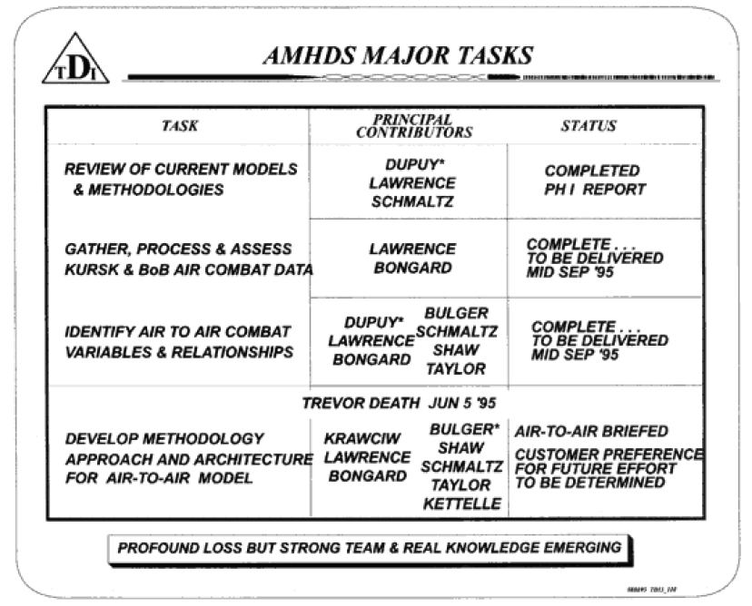
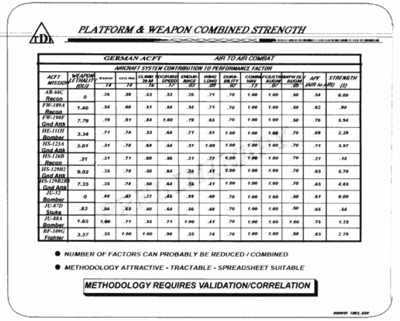
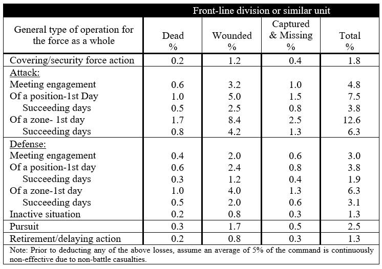
The first of Trevor Dupuy’s Timeless Verities of Combat is:

Offensive action is essential to positive combat results.

As he explained in Understanding War (1987):

This is like saying, “A team can’t score in football unless it has the ball.” Although subsequent verities stress the strength, value, and importance of defense, this should not obscure the essentiality of offensive action to ultimate combat success. Even in instances where a defensive strategy might conceivably assure a favorable war outcome—as was the case of the British against Napoleon, and as the Confederacy attempted in the American Civil War—selective employment of offensive tactics and operations is required if the strategic defender is to have any chance of final victory. [pp. 1-2]

The offensive has long been a staple element of the principles of war. From the 1954 edition of the U.S. Army Field Manual FM 100-5, Field Service Regulations, Operations:

71. Offensive

Only offensive action achieves decisive results. Offensive action permits the commander to exploit the initiative and impose his will on the enemy. The defensive may be forced on the commander, but it should be deliberately adopted only as a temporary expedient while awaiting an opportunity for offensive action or for the purpose of economizing forces on a front where a decision is not sought. Even on the defensive the commander seeks every opportunity to seize the initiative and achieve decisive results by offensive action. [Original emphasis]

Interestingly enough, the offensive no longer retains its primary place in current Army doctrinal thought. The Army consigned its list of the principles of war to an appendix in the 2008 edition of FM 3-0 Operations and omitted them entirely from the 2017 revision. As the current edition of FM 3-0 Operations lays it out, the offensive is now placed on the same par as the defensive and stability operations:

Unified land operations are simultaneous offensive, defensive, and stability or defense support of civil authorities’ tasks to seize, retain, and exploit the initiative to shape the operational environment, prevent conflict, consolidate gains, and win our Nation’s wars as part of unified action (ADRP 3-0)…

At the heart of the Army’s operational concept is decisive action. Decisive action is the continuous, simultaneous combinations of offensive, defensive, and stability or defense support of civil authorities tasks (ADRP 3-0). During large-scale combat operations, commanders describe the combinations of offensive, defensive, and stability tasks in the concept of operations. As a single, unifying idea, decisive action provides direction for an entire operation. [p. I-16; original emphasis]

It is perhaps too easy to read too much into this change in emphasis. On the very next page, FM 3-0 describes offensive “tasks” thusly:

Offensive tasks are conducted to defeat and destroy enemy forces and seize terrain, resources, and population centers. Offensive tasks impose the commander’s will on the enemy. The offense is the most direct and sure means of seizing and exploiting the initiative to gain physical and cognitive advantages over an enemy. In the offense, the decisive operation is a sudden, shattering action that capitalizes on speed, surprise, and shock effect to achieve the operation’s purpose. If that operation does not destroy or defeat the enemy, operations continue until enemy forces disintegrate or retreat so they no longer pose a threat. Executing offensive tasks compels an enemy to react, creating or revealing additional weaknesses that an attacking force can exploit. [p. I-17]

The change in emphasis likely reflects recent U.S. military experience where decisive action has not yielded much in the way of decisive outcomes, as is mentioned in FM 3-0’s introduction. Joint force offensives in 2001 and 2003 “achieved rapid initial military success but no enduring political outcome, resulting in protracted counterinsurgency campaigns.” The Army now anticipates a future operating environment where joint forces can expect to “work together and with unified action partners to successfully prosecute operations short of conflict, prevail in large-scale combat operations, and consolidate gains to win enduring strategic outcomes” that are not necessarily predicated on offensive action alone. We may have to wait for the next edition of FM 3-0 to see if the Army has drawn valid conclusions from the recent past or not.

Was Kursk the Largest Tank Battle in History?

[This post was originally published on 3 April 2017.]

Displayed across the top of my book is the phrase “Largest Tank Battle in History.” Apparently some people dispute that.

What they put forth as the largest tank battle in history is the Battle of Brody in 23-30 June 1941. This battle occurred right at the start of the German invasion of the Soviet Union and consisted of two German corps attacking five Soviet corps in what is now Ukraine. This rather confused affair pitted between 750 to 1,000 German tanks against 3,500 to 5,000 Soviet tanks. Only 3,000 Soviet tanks made it to the battlefield according to Glantz (see video at 16:00). The German won with losses of around a 100 to 200 tanks. Sources vary on this, and I have not taken the time to sort this out (so many battles, so little time). So, total tanks involved are from 3,750 to up to 6,000, with the lower figure appearing to be more correct.

Now, is this really a larger tank battle than the Battle of Kursk? My book covers only the southern part of the German attack that started on 4 July and ended 17 July. This offensive involved five German corps (including three Panzer corps consisting of nine panzer and panzer grenadier divisions) and they faced seven Soviet Armies (including two tank armies and a total of ten tank and mechanized corps).

My tank counts for the southern attack staring 4 July 1943 was 1,707 German tanks (1,709 depending if you count the two Panthers that caught fire on the move up there). The Soviets at 4 July in the all formations that would eventually get involved has 2,775 tanks with 1,664 tanks in the Voronezh Front at the start of the battle. Our count of total committed tanks is slightly higher, 1,749 German and 2,978 Soviet. This includes tanks that were added during the two weeks of battle and mysterious adjustments to strength figures that we cannot otherwise explain. This is 4,482 or 4,727 tanks. So depending on which Battle of Brody figures being used, and whether all the Soviet tanks were indeed ready-for-action and committed to the battle, then the Battle of Brody might be larger than the attack in the southern part of the Kursk salient. On the other hand, it probably is not.

But, this was just one part of the Battle of Kursk. To the north was the German attack from the Orel salient that was about two-thirds the size of the attack in the south. It consisted of the Ninth Army with five corps and six German panzer divisions. This offensive fizzled at the Battle of Ponyiri on 12 July.

The third part to the Battle of Kursk began on 12 July the Western and Bryansk Fronts launched an offensive on the north side of the Orel salient. A Soviet Front is equivalent to an army group and this attack initially consisted of five armies and included four Soviet tank corps. This was a major attack that added additional forces as it developed and went on until 23 August.

The final part of the Battle of Kursk was the counter-offensive in the south by Voronezh, Southwestern and Steppe Fronts that started on 3 August, took Kharkov and continued until 23 August. The Soviet forces involved here were larger than the forces involved in the original defensive effort, with the Voronezh Front now consisting of eight armies, the Steppe Front consisting of three armies, and there being one army contributed by the Southwestern Front to this attack.

The losses in these battles were certainly more significant for the Germans than at the Battle of Brody. For example, in the southern offensive by our count the Germans lost 1,536 tanks destroyed, damaged or broken down. The Soviets lost 2,471 tanks destroyed, damaged or broken down. This compares to 100-200 German tanks lost at Brody and the Soviet tank losses are even more nebulous, but the figure of 2,648 has been thrown out there.

So, total tanks involved in the German offensive in the south were 4,482 or 4,727 and this was just one of four parts of the Battle of Kursk. Losses were higher than for Brody (and much higher for the Germans). Obviously, the Battle of Kursk was a larger tank battle than the Battle of Brody.

What some people are comparing the Battle of Brody to is the Battle of Prokhorovka. This was a one- to five-day event during the German offensive in the south that included the German SS Panzer Corps and in some people’s reckoning, all of the III Panzer Corps and the 11th Panzer Division from the XLVIII Panzer Corps. So, the Battle of Brody may well be a larger tank battle than the Battle of Prokhorovka, but it was not a larger tank battle than the Battle of Kursk. I guess it depends all in how you define the battles.

Some links on Battle of Brody:

https://en.wikipedia.org/wiki/Battle_of_Brody_(1941)

http://warisboring.com/the-biggest-tank-battle-in-history-wasnt-at-kursk/

https://www.youtube.com/watch?v=5qkmO7tm8AU

What Is A Breakpoint?

French retreat from Russia in 1812 by Illarion Mikhailovich Pryanishnikov (1812) [Wikipedia]

After discussing with Chris the series of recent posts on the subject of breakpoints, it seemed appropriate to provide a better definition of exactly what a breakpoint is.

Dorothy Kneeland Clark was the first to define the notion of a breakpoint in her study, Casualties as a Measure of the Loss of Combat Effectiveness of an Infantry Battalion (Operations Research Office, The Johns Hopkins University: Baltimore, 1954). She found it was not quite as clear-cut as it seemed and the working definition she arrived at was based on discussions and the specific combat outcomes she found in her data set [pp 9-12].

DETERMINATION OF BREAKPOINT

The following definitions were developed out of many discussions. A unit is considered to have lost its combat effectiveness when it is unable to carry out its mission. The onset of this inability constitutes a breakpoint. A unit’s mission is the objective assigned in the current operations order or any other instructional directive, written or verbal. The objective may be, for example, to attack in order to take certain positions, or to defend certain positions. 

How does one determine when a unit is unable to carry out its mission? The obvious indication is a change in operational directive: the unit is ordered to stop short of its original goal, to hold instead of attack, to withdraw instead of hold. But one or more extraneous elements may cause the issue of such orders: 

(1) Some other unit taking part in the operation may have lost its combat effectiveness, and its predicament may force changes, in the tactical plan. For example the inability of one infantry battalion to take a hill may require that the two adjoining battalions be stopped to prevent exposing their flanks by advancing beyond it. 

(2) A unit may have been assigned an objective on the basis of a G-2 estimate of enemy weakness which, as the action proceeds, proves to have been over-optimistic. The operations plan may, therefore, be revised before the unit has carried out its orders to the point of losing combat effectiveness. 

(3) The commanding officer, for reasons quite apart from the tactical attrition, may change his operations plan. For instance, General Ridgway in May 1951 was obliged to cancel his plans for a major offensive north of the 38th parallel in Korea in obedience to top level orders dictated by political considerations. 

(4) Even if the supposed combat effectiveness of the unit is the determining factor in the issuance of a revised operations order, a serious difficulty in evaluating the situation remains. The commanding officer’s decision is necessarily made on the basis of information available to him plus his estimate of his unit’s capacities. Either or both of these bases may be faulty. The order may belatedly recognize a collapse which has in factor occurred hours earlier, or a commanding officer may withdraw a unit which could hold for a much longer time. 

It was usually not hard to discover when changes in orders resulted from conditions such as the first three listed above, but it proved extremely difficult to distinguish between revised orders based on a correct appraisal of the unit’s combat effectiveness and those issued in error. It was concluded that the formal order for a change in mission cannot be taken as a definitive indication of the breakpoint of a unit. It seemed necessary to go one step farther and search the records to learn what a given battalion did regardless of provisions in formal orders… 

CATEGORIES OF BREAKPOINTS SELECTED 

In the engagements studied the following categories of breakpoint were finally selected: 

Category of Breakpoint 

No. Analyzed 

I. Attack [Symbol] rapid reorganization [Symbol] attack 

9 

II. Attack [Symbol] defense (no longer able to attack without a few days of recuperation and reinforcement 

21 

III. Defense [Symbol] withdrawal by order to a secondary line 

13 

IV. Defense [Symbol] collapse 

5 

Disorganization and panic were taken as unquestionable evidence of loss of combat effectiveness. It appeared, however, that there were distinct degrees of magnitude in these experiences. In addition to the expected breakpoints at attack [Symbol] defense and defense [Symbol] collapse, a further category, I, seemed to be indicated to include situations in which an attacking battalion was ‘pinned down” or forced to withdraw in partial disorder but was able to reorganize in 4 to 24 hours and continue attacking successfully. 

Category II includes (a) situations in which an attacking battalion was ordered into the defensive after severe fighting or temporary panic; (b) situations in which a battalion, after attacking successfully, failed to gain ground although still attempting to advance and was finally ordered into defense, the breakpoint being taken as occurring at the end of successful advance. In other words, the evident inability of the unit to fulfill its mission was used as the criterion for the breakpoint whether orders did or did not recognize its inability. Battalions after experiencing such a breakpoint might be able to recuperate in a few days to the point of renewing successful attack or might be able to continue for some time in defense. 

The sample of breakpoints coming under category IV, defense [Symbol] collapse, proved to be very small (5) and unduly weighted in that four of the examples came from the same engagement. It was, therefore, discarded as probably not representative of the universe of category IV breakpoints,* and another category (III) was added: situations in which battalions on the defense were ordered withdrawn to a quieter sector. Because only those instances were included in which the withdrawal orders appeared to have been dictated by the condition of the unit itself, it is believed that casualty levels for this category can be regarded as but slightly lower than those associated with defense [Symbol] collapse. 

In both categories II and III, “‘defense” represents an active situation in which the enemy is attacking aggressively. 

* It had been expected that breakpoints in this category would be associated with very high losses. Such did not prove to be the case. In whatever way the data were approached, most of the casualty averages were only slightly higher than those associated with category II (attack [Symbol] defense), although the spread in data was wider. It is believed that factors other than casualties, such as bad weather, difficult terrain, and heavy enemy artillery fire undoubtedly played major roles in bringing about the collapse in the four units taking part in the same engagement. Furthermore, the casualty figures for the four units themselves is in question because, as the situation deteriorated, many of the men developed severe cases of trench foot and combat exhaustion, but were not evacuated, as they would have been in a less desperate situation, and did not appear in the casualty records until they had made their way to the rear after their units had collapsed.

In 1987-1988, Trevor Dupuy and colleagues at Data Memory Systems, Inc. (DMSi), Janice Fain, Rich Anderson, Gay Hammerman, and Chuck Hawkins sought to create a broader, more generally applicable definition for breakpoints for the study, Forced Changes of Combat Posture (DMSi, Fairfax, VA, 1988) [pp. I-2-3]

The combat posture of a military force is the immediate intention of its commander and troops toward the opposing enemy force, together with the preparations and deployment to carry out that intention. The chief combat postures are attack, defend, delay, and withdraw.

A change in combat posture (or posture change) is a shift from one posture to another, as, for example, from defend to attack or defend to withdraw. A posture change can be either voluntary or forced. 

A forced posture change (FPC) is a change in combat posture by a military unit that is brought about, directly or indirectly, by enemy action. Forced posture changes are characteristically and almost always changes to a less aggressive posture. The most usual FPCs are from attack to defend and from defend to withdraw (or retrograde movement). A change from withdraw to combat ineffectiveness is also possible. 

Breakpoint is a term sometimes used as synonymous with forced posture change, and sometimes used to mean the collapse of a unit into ineffectiveness or rout. The latter meaning is probably more common in general usage, while forced posture change is the more precise term for the subject of this study. However, for brevity and convenience, and because this study has been known informally since its inception as the “Breakpoints” study, the term breakpoint is sometimes used in this report. When it is used, it is synonymous with forced posture change.

Hopefully this will help clarify the previous discussions of breakpoints on the blog.

U.S. Army Invests In Revitalizing Long Range Precision Fires Capabilities

U.S. Marines from the The 11th MEU fire their M777 Lightweight 155mm Howitzer during Exercise Alligator Dagger, Dec. 18, 2016. (U.S. Marine Corps/Lance Cpl. Zachery C. Laning/Military.com)

In 2016, Michael Jacobson and Robert H. Scales amplified a warning that after years of neglect during the counterinsurgency war in Iraq and Afghanistan, the U.S. was falling behind potential adversaries in artillery and long range precision fires capabilities. The U.S. Army had already taken note of the performance of Russian artillery in Ukraine, particularly the strike at Zelenopillya in 2014.

Since then, the U.S. Army and Marine Corps have started working on a new Multi-Domain Battle concept aimed at countering the anti-access/area denial (A2/AD) capabilities of potential foes. In 2017, U.S. Army Chief of Staff General Mark Milley made rapid improvement in long range precision fires capabilities the top priority for the service’s modernization effort. It currently aims to field new field artillery, rocket, and missile weapons capable of striking at distances from 70 to 500 kilometers – double the existing ranges – within five years.

The value of ground-based long-range precision fires has been demonstrated recently by the effectiveness of U.S. artillery support, particularly U.S. Army and Marine Corps 155mm howitzers, for Iraqi security forces in retaking Mosul, Syrian Democratic Forces assaulting Raqaa, and in protection of Syrian Kurds being attacked by Russian mercenaries and Syrian regime forces.

According to Army historian Luke O’Brian, the Fiscal Year 2019 Defense budget includes funds to buy 28,737 XM1156 Precision Guided Kit (PGK) 155mm howitzer munitions, which includes replacements for the 6,269 rounds expended during Operation INHERENT RESOLVE. O’Brian also notes that the Army will also buy 2,162 M982 Excalibur 155mm rounds in 2019 and several hundred each in following years.

In addition, in an effort to reduce the dependence on potentially vulnerable Global Positioning System (GPS) satellite networks for precision fires capabilities, the Army has awarded a contract to BAE Systems to develop Precision Guided Kit-Modernization (PGK-M) rounds with internal navigational capacity.

While the numbers appear large at first glance, data on U.S. artillery expenditures in Operation DESERT STORM and IRAQI FREEDOM (also via Luke O’Brian) shows just how much the volume of long-range fires has changed just since 1991. For the U.S. at least, precision fires have indeed replaced mass fires on the battlefield.

Breakpoints in U.S. Army Doctrine

U.S. Army prisoners of war captured by German forces during the Battle of the Bulge in 1944. [Wikipedia]

One of the least studied aspects of combat is battle termination. Why do units in combat stop attacking or defending? Shifts in combat posture (attack, defend, delay, withdrawal) are usually voluntary, directed by a commander, but they can also be involuntary, as a result of direct or indirect enemy action. Why do involuntary changes in combat posture, known as breakpoints, occur?

As Chris pointed out in a previous post, the topic of breakpoints has only been addressed by two known studies since 1954. Most existing military combat models and wargames address breakpoints in at least a cursory way, usually through some calculation based on personnel casualties. Both of the breakpoints studies suggest that involuntary changes in posture are seldom related to casualties alone, however.

Current U.S. Army doctrine addresses changes in combat posture through discussions of culmination points in the attack, and transitions from attack to defense, defense to counterattack, and defense to retrograde. But these all pertain to voluntary changes, not breakpoints.

Army doctrinal literature has little to say about breakpoints, either in the context of friendly forces or potential enemy combatants. The little it does say relates to the effects of fire on enemy forces and is based on personnel and material attrition.

According to ADRP 1-02 Terms and Military Symbols, an enemy combat unit is considered suppressed after suffering 3% personnel casualties or material losses, neutralized by 10% losses, and destroyed upon sustaining 30% losses. The sources and methodology for deriving these figures is unknown, although these specific terms and numbers have been a part of Army doctrine for decades.

The joint U.S. Army and U.S. Marine Corps vision of future land combat foresees battlefields that are highly lethal and demanding on human endurance. How will such a future operational environment affect combat performance? Past experience undoubtedly offers useful insights but there seems to be little interest in seeking out such knowledge.

Trevor Dupuy criticized the U.S. military in the 1980s for its lack of understanding of the phenomenon of suppression and other effects of fire on the battlefield, and its seeming disinterest in studying it. Not much appears to have changed since then.

The Dupuy Air Campaign Model (DACM)

[The article below is reprinted from the April 1997 edition of The International TNDM Newsletter. A description of the TDI Air Model Historical Data Study can be found here.]

The Dupuy Air Campaign Model
by Col. Joseph A. Bulger, Jr., USAF, Ret.

The Dupuy Institute, as part of the DACM [Dupuy Air Campaign Model], created a draft model in a spreadsheet format to show how such a model would calculate attrition. Below are the actual printouts of the “interim methodology demonstration,” which shows the types of inputs, outputs, and equations used for the DACM. The spreadsheet was created by Col. Bulger, while many of the formulae were the work of Robert Shaw.

The Dupuy Institute Air Model Historical Data Study

British Air Ministry aerial combat diagram that sought to explain how the RAF had fought off the Luftwaffe. [World War II Today]

[The article below is reprinted from the April 1997 edition of The International TNDM Newsletter.]

Air Model Historical Data Study
by Col. Joseph A. Bulger, Jr., USAF, Ret

The Air Model Historical Study (AMHS) was designed to lead to the development of an air campaign model for use by the Air Command and Staff College (ACSC). This model, never completed, became known as the Dupuy Air Campaign Model (DACM). It was a team effort led by Trevor N. Dupuy and included the active participation of Lt. Col. Joseph Bulger, Gen. Nicholas Krawciw, Chris Lawrence, Dave Bongard, Robert Schmaltz, Robert Shaw, Dr. James Taylor, John Kettelle, Dr. George Daoust and Louis Zocchi, among others. After Dupuy’s death, I took over as the project manager.

At the first meeting of the team Dupuy assembled for the study, it became clear that this effort would be a serious challenge. In his own style, Dupuy was careful to provide essential guidance while, at the same time, cultivating a broad investigative approach to the unique demands of modeling for air combat. It would have been no surprise if the initial guidance established a focus on the analytical approach, level of aggregation, and overall philosophy of the QJM [Quantified Judgement Model] and TNDM [Tactical Numerical Deterministic Model]. It was clear that Trevor had no intention of steering the study into an air combat modeling methodology based directly on QJM/TNDM. To the contrary, he insisted on a rigorous derivation of the factors that would permit the final choice of model methodology.

At the time of Dupuy’s death in June 1995, the Air Model Historical Data Study had reached a point where a major decision was needed. The early months of the study had been devoted to developing a consensus among the TDI team members with respect to the factors that needed to be included in the model. The discussions tended to highlight three areas of particular interest—factors that had been included in models currently in use, the limitations of these models, and the need for new factors (and relationships) peculiar to the properties and dynamics of the air campaign. Team members formulated a family of relationships and factors, but the model architecture itself was not investigated beyond the surface considerations.

Despite substantial contributions from team members, including analytical demonstrations of selected factors and air combat relationships, no consensus had been achieved. On the contrary, there was a growing sense of need to abandon traditional modeling approaches in favor of a new application of the “Dupuy Method” based on a solid body of air combat data from WWII.

The Dupuy approach to modeling land combat relied heavily on the ratio of force strengths (largely determined by firepower as modified by other factors). After almost a year of investigations by the AMHDS team, it was beginning to appear that air combat differed in a fundamental way from ground combat. The essence of the difference is that in air combat, the outcome of the maneuver battle for platform position must be determined before the firepower relationships may be brought to bear on the battle outcome.

At the time of Dupuy’s death, it was apparent that if the study contract was to yield a meaningful product, an immediate choice of analysis thrust was required. Shortly prior to Dupuy’s death, I and other members of the TDI team recommended that we adopt the overall approach, level of aggregation, and analytical complexity that had characterized Dupuy’s models of land combat. We also agreed on the time-sequenced predominance of the maneuver phase of air combat. When I was asked to take the analytical lead for the contact in Dupuy’s absence, I was reasonably confident that there was overall agreement.

In view of the time available to prepare a deliverable product, it was decided to prepare a model using the air combat data we had been evaluating up to that point—June 1995. Fortunately, Robert Shaw had developed a set of preliminary analysis relationships that could be used in an initial assessment of the maneuver/firepower relationship. In view of the analytical, logistic, contractual, and time factors discussed, we decided to complete the contract effort based on the following analytical thrust:

  1. The contract deliverable would be based on the maneuver/firepower analysis approach as currently formulated in Robert Shaw’s performance equations;
  2. A spreadsheet formulation of outcomes for selected (Battle of Britain) engagements would be presented to the customer in August 1995;
  3. To the extent practical, a working model would be provided to the customer with suggestions for further development.

During the following six weeks, the demonstration model was constructed. The model (programmed for a Lotus 1-2-3 style spreadsheet formulation) was developed, mechanized, and demonstrated to ACSC in August 1995. The final report was delivered in September of 1995.

The working model demonstrated to ACSC in August 1995 suggests the following observations:

  • A substantial contribution to the understanding of air combat modeling has been achieved.
  • While relationships developed in the Dupuy Air Combat Model (DACM) are not fully mature, they are analytically significant.
  • The approach embodied in DACM derives its authenticity from the famous “Dupuy Method” thus ensuring its strong correlations with actual combat data.
  • Although demonstrated only for air combat in the Battle of Britain, the methodology is fully capable of incorporating modem technology contributions to sensor, command and control, and firepower performance.
  • The knowledge base, fundamental performance relationships, and methodology contributions embodied in DACM are worthy of further exploration. They await only the expression of interest and a relatively modest investment to extend the analysis methodology into modem air combat and the engagements anticipated for the 21st Century.

One final observation seems appropriate. The DACM demonstration provided to ACSC in August 1995 should not be dismissed as a perhaps interesting, but largely simplistic approach to air combat modeling. It is a significant contribution to the understanding of air combat relationships that will prevail in the 21st Century. The Dupuy Institute is convinced that further development of DACM makes eminent good sense. An exploitation of the maneuver and firepower relationships already demonstrated in DACM will provide a valid basis for modeling air combat with modern technology sensors, control mechanisms, and weapons. It is appropriate to include the Dupuy name in the title of this latest in a series of distinguished combat models. Trevor would be pleased.

‘Love’s Tables’: U.S. War Department Casualty Estimation in World War II

The same friend of TDI who asked about ‘Evett’s Rates,” the British casualty estimation methodology during World War II, also mentioned that the work of Albert G. Love III was now available on-line. Rick Atkinson also referenced “Love’s Tables” in The Guns At Last Light.

In 1931, Lieutenant Colonel (later Brigadier General) Love, then a Medical Corps physician in the U.S. Army Medical Field Services School, published a study of American casualty data in the recent Great War, titled “War Casualties.”[1] This study was likely the source for tables used for casualty estimation by the U.S. Army through 1944.[2]

Love, who had no advanced math or statistical training, undertook his study with the support of the Army Surgeon General, Merritte W. Ireland, and initial assistance from Dr. Lowell J. Reed, a professor of biostatistics at John Hopkins University. Love’s posting in the Surgeon General’s Office afforded him access to an array of casualty data collected from the records of the American Expeditionary Forces in France, as well as data from annual Surgeon General reports dating back to 1819, the official medical history of the U.S. Civil War, and U.S. general population statistics.

Love’s research was likely the basis for rate tables for calculating casualties that first appeared in the 1932 edition of the War Department’s Staff Officer’s Field Manual.[3]

Battle Casualties, including Killed, in Percent of Unit Strength, Staff Officer’s Field Manual (1932).

The 1932 Staff Officer’s Field Manual estimation methodology reflected Love’s sophisticated understanding of the factors influencing combat casualty rates. It showed that both the resistance and combat strength (and all of the factors that comprised it) of the enemy, as well as the equipment and state of training and discipline of the friendly troops had to be taken into consideration. The text accompanying the tables pointed out that loss rates in small units could be quite high and variable over time, and that larger formations took fewer casualties as a fraction of overall strength, and that their rates tended to become more constant over time. Casualties were not distributed evenly, but concentrated most heavily among the combat arms, and in the front-line infantry in particular. Attackers usually suffered higher loss rates than defenders. Other factors to be accounted for included the character of the terrain, the relative amount of artillery on each side, and the employment of gas.

The 1941 iteration of the Staff Officer’s Field Manual, now designated Field Manual (FM) 101-10[4], provided two methods for estimating battle casualties. It included the original 1932 Battle Casualties table, but the associated text no longer included the section outlining factors to be considered in calculating loss rates. This passage was moved to a note appended to a new table showing the distribution of casualties among the combat arms.

Rather confusingly, FM 101-10 (1941) presented a second table, Estimated Daily Losses in Campaign of Personnel, Dead and Evacuated, Per 1,000 of Actual Strength. It included rates for front line regiments and divisions, corps and army units, reserves, and attached cavalry. The rates were broken down by posture and tactical mission.

Estimated Daily Losses in Campaign of Personnel, Dead and Evacuated, Per 1,000 of Actual Strength, FM 101-10 (1941)

The source for this table is unknown, nor the method by which it was derived. No explanatory text accompanied it, but a footnote stated that “this table is intended primarily for use in school work and in field exercises.” The rates in it were weighted toward the upper range of the figures provided in the 1932 Battle Casualties table.

The October 1943 edition of FM 101-10 contained no significant changes from the 1941 version, except for the caveat that the 1932 Battle Casualties table “may or may not prove correct when applied to the present conflict.”

The October 1944 version of FM 101-10 incorporated data obtained from World War II experience.[5] While it also noted that the 1932 Battle Casualties table might not be applicable, the experiences of the U.S. II Corps in North Africa and one division in Italy were found to be in agreement with the table’s division and corps loss rates.

FM 101-10 (1944) included another new table, Estimate of Battle Losses for a Front-Line Division (in % of Actual Strength), meaning that it now provided three distinct methods for estimating battle casualties.

Estimate of Battle Losses for a Front-Line Division (in % of Actual Strength), FM 101-10 (1944)

Like the 1941 Estimated Daily Losses in Campaign table, the sources for this new table were not provided, and the text contained no guidance as to how or when it should be used. The rates it contained fell roughly within the span for daily rates for severe (6-8%) to maximum (12%) combat listed in the 1932 Battle Casualty table, but would produce vastly higher overall rates if applied consistently, much higher than the 1932 table’s 1% daily average.

FM 101-10 (1944) included a table showing the distribution of losses by branch for the theater based on experience to that date, except for combat in the Philippine Islands. The new chart was used in conjunction with the 1944 Estimate of Battle Losses for a Front-Line Division table to determine daily casualty distribution.

Distribution of Battle Losses–Theater of Operations, FM 101-10 (1944)

The final World War II version of FM 101-10 issued in August 1945[6] contained no new casualty rate tables, nor any revisions to the existing figures. It did finally effectively invalidate the 1932 Battle Casualties table by noting that “the following table has been developed from American experience in active operations and, of course, may not be applicable to a particular situation.” (original emphasis)

NOTES

[1] Albert G. Love, War Casualties, The Army Medical Bulletin, No. 24, (Carlisle Barracks, PA: 1931)

[2] This post is adapted from TDI, Casualty Estimation Methodologies Study, Interim Report (May 2005) (Altarum) (pp. 314-317).

[3] U.S. War Department, Staff Officer’s Field Manual, Part Two: Technical and Logistical Data (Government Printing Office, Washington, D.C., 1932)

[4] U.S. War Department, FM 101-10, Staff Officer’s Field Manual: Organization, Technical and Logistical Data (Washington, D.C., June 15, 1941)

[5] U.S. War Department, FM 101-10, Staff Officer’s Field Manual: Organization, Technical and Logistical Data (Washington, D.C., October 12, 1944)

[6] U.S. War Department, FM 101-10 Staff Officer’s Field Manual: Organization, Technical and Logistical Data (Washington, D.C., August 1, 1945)

‘Evett’s Rates’: British War Office Wastage Tables

Stretcher bearers of the East Surrey Regiment, with a Churchill tank of the North Irish Horse in the background, during the attack on Longstop Hill, Tunisia, 23 April 1943. [Imperial War Museum/Wikimedia]

A friend of TDI queried us recently about a reference in Rick Atkinson’s The Guns at Last Light: The War in Western Europe, 1944-1945 to a British casualty estimation methodology known as “Evett’s Rates.” There are few references to Evett’s Rates online, but as it happens, TDI did find out some details about them for a study on casualty estimation. [1]

British Army staff officers during World War II and the 1950s used a set of look-up tables which listed expected monthly losses in percentage of strength for various arms under various combat conditions. The origin of the tables is not known, but they were officially updated twice, in 1942 by a committee chaired by Major General Evett, and in 1951-1955 by the Army Operations Research Group (AORG).[2]

The methodology was based on staff predictions of one of three levels of operational activity, “Intense,” “Normal,” and “Quiet.” These could be applied to an entire theater, or to individual divisions. The three levels were defined the same way for both the Evett Committee and AORG rates:

The rates were broken down by arm and rank, and included battle and nonbattle casualties.

Rates of Personnel Wastage Including Both Battle and Non-battle Casualties According to the Evett Committee of 1942. (Percent per 30 days).

The Evett Committee rates were criticized during and after the war. After British forces suffered twice the anticipated casualties at Anzio, the British 21st Army Group applied a “double intense rate” which was twice the Evett Committee figure and intended to apply to assaults. When this led to overestimates of casualties in Normandy, the double intense rate was discarded.

From 1951 to 1955, AORG undertook a study of casualty rates in World War II. Its analysis was based on casualty data from the following campaigns:

  • Northwest Europe, 1944
    • 6-30 June – Beachhead offensive
    • 1 July-1 September – Containment and breakout
    • 1 October-30 December – Semi-static phase
    • 9 February to 6 May – Rhine crossing and final phase
  • Italy, 1944
    • January to December – Fighting a relatively equal enemy in difficult country. Warfare often static.
    • January to February (Anzio) – Beachhead held against severe and well-conducted enemy counter-attacks.
  • North Africa, 1943
    • 14 March-13 May – final assault
  • Northwest Europe, 1940
    • 10 May-2 June – Withdrawal of BEF
  • Burma, 1944-45

From the first four cases, the AORG study calculated two sets of battle casualty rates as percentage of strength per 30 days. “Overall” rates included KIA, WIA, C/MIA. “Apparent rates” included these categories but subtracted troops returning to duty. AORG recommended that “overall” rates be used for the first three months of a campaign.

The Burma campaign data was evaluated differently. The analysts defined a “force wastage” category which included KIA, C/MIA, evacuees from outside the force operating area and base hospitals, and DNBI deaths. “Dead wastage” included KIA, C/MIA, DNBI dead, and those discharged from the Army as a result of injuries.

The AORG study concluded that the Evett Committee underestimated intense loss rates for infantry and armor during periods of very hard fighting and overestimated casualty rates for other arms. It recommended that if only one brigade in a division was engaged, two-thirds of the intense rate should be applied, if two brigades were engaged the intense rate should be applied, and if all brigades were engaged then the intense rate should be doubled. It also recommended that 2% extra casualties per month should be added to all the rates for all activities should the forces encounter heavy enemy air activity.[1]

The AORG study rates were as follows:

Recommended AORG Rates of Personnel Wastage. (Percent per 30 days).

If anyone has further details on the origins and activities of the Evett Committee and AORG, we would be very interested in finding out more on this subject.

NOTES

[1] This post is adapted from The Dupuy Institute, Casualty Estimation Methodologies Study, Interim Report (May 2005) (Altarum) (pp. 51-53).

[2] Rowland Goodman and Hugh Richardson. “Casualty Estimation in Open and Guerrilla Warfare.” (London: Directorate of Science (Land), U.K. Ministry of Defence, June 1995.), Appendix A.

Drones And The U.S. Navy

An X-47 Unmanned Combat Air System (UCAS) drone lands on the USS Theodore Roosevelt during a test in 2014. [Breaking Defense]

Preamble & Warning (P&W): Please forgive me, this is an acronym heavy post.

In May 2013, the U.S. Navy (USN) reached milestones by having a “drone,” or unmanned aerial vehicle (UAV) land and take-off from an aircraft carrier. This was a significant achievement in aviation, and heralded an era of combat UAVs (UCAV) being integrated into carrier air wings (CVW). This vehicle, the X-47B, was built by Northrup Grumman, under the concept of a carrier-based stealthy strike vehicle.

Ultimately, after almost three years, their decision was announced:

On 1 February 2016, after many delays over whether the [Unmanned Carrier-Launched Airborne Surveillance and Strike] UCLASS would specialize in strike or intelligence, surveillance and reconnaissance (ISR) roles, it was reported that a significant portion of the UCLASS effort would be directed to produce a Super Hornet-sized carrier-based aerial refueling tanker as the Carrier-Based Aerial-Refueling System (CBARS), with ‘a little ISR’ and some capabilities for communications relay, and strike capabilities put off to a future version of the aircraft. In July 2016, it was officially named ‘MQ-25A Stingray’.

The USN, who had just proven that they can add a stealthy UCAV to carrier flight deck operations, decided to put this new capability on the shelf, and instead refocus the efforts of the aerospace defense industry on a brand new requirement, namely …

For mission tanking, the threshold requirement is offloading 14,000 lb. of fuel to aviation assets at 500 nm from the ship, thereby greatly extending the range of the carrier air wing, including the Lockheed Martin F-35C and Boeing F/A-18 Super Hornet. The UAV must also be able to integrate with the Nimitz-class carriers, being able to safely launch and recover and not take up more space than is allocated for storage, maintenance and repairs.

Boeing has fashioned part of St. Louis Lambert International Airport into an aircraft carrier deck, complete with a mock catapult system. [Boeing]

Why did they do this?

The Pentagon apparently made this program change in order to address the Navy’s expected fighter shortfall by directing funds to buy additional F/A-18E/F Super Hornets and accelerate purchases and development of the F-35C. Having the CBARS as the first carrier-based UAV provides a less complex bridge to the future F/A-XX, should it be an autonomous strike platform. It also addresses the carriers’ need for an organic refueling aircraft, proposed as a mission for the UCLASS since 2014, freeing up the 20–30 percent of Super Hornets performing the mission in a more capable and cost effective manner than modifying the F-35, V-22 Osprey, and E-2D Hawkeye, or bringing the retired S-3 Viking back into service.

Notice within this quote the supposition that the F/A-XX would be an autonomous strike platform. This program was originally a USN-specific program to build a next-generation platform to perform both strike and air superiority missions, much like the F/A-18 aircraft are “swing role.” The US Air Force (USAF) had a separate program for a next generation air superiority aircraft called the F-X. These programs were combined by the Department of Defense (DoD) into the Next Generation Air Dominance (NGAD) program. We can tell from the name of this program that it is clearly focused on the air superiority mission, as compared to the balance of strike and superiority, implicit in the USN program.

Senator John McCain, chairman of the Senate Armed Services Committee (SASC), wrote a letter to then Secretary of Defense Ash Carter, on 2015-03-24, stating, “I strongly believe that the Navy’s first operational unmanned combat aircraft must be capable of performing a broad range of missions in contested environments as part of the carrier air wing, including precision strike as well as [ISR].” This is effectively an endorsement of the X-47B, and quite unlike the MQ-25.

I’m in agreement with Senator McCain on this. I think that a great deal of experience could have been gained by continuing the development and test of the X-47B, and possibly deploying the vehicle to the fleet.

The Navy hinted at the possibility of using the UCLASS in air-to-air engagements as a ‘flying missile magazine’ to supplement the F/A-18 Super Hornet and F-35C Lightning II as a type of ‘robotic wingman.’ Its weapons bay could be filled with AIM-120 AMRAAMs and be remotely operated by an E-2D Hawkeye or F-35C flight leader, using their own sensors and human judgment to detect, track, and direct the UAV to engage an enemy aircraft. The Navy’s Naval Integrated Fire Control-Counter Air (NIFC-CA) concept gives a common picture of the battle space to multiple air platforms through data-links, where any aircraft could fire on a target in their range that is being tracked by any sensor, so the forward deployed UCLASS would have its missiles targeted by another controller. With manned-unmanned teaming for air combat, a dedicated unmanned supersonic fighter may not be developed, as the greater cost of high-thrust propulsion and an airframe of similar size to a manned fighter would deliver a platform with comparable operating costs and still without an ability to engage on its own.

Indeed, the German Luftwaffe has completed an air combat concept study, stating that the fighter of the 2040’s will be a “stealthy drone herder”:

Interestingly the twin-engine, twin-tail stealth design would be a twin-seat design, according to Alberto Gutierrez, Head of Eurofighter Programme, Airbus DS. The second crewmember may be especially important for the FCAS concept of operations, which would see it operate in a wider battle network, potentially as a command and control asset or UCAV/UAV mission commander.

Instead, the USN has decided to banish the drones into the tanker and light ISR roles, to focus on having more Super Hornets available, and move towards integrating the F-35C into the CVW. I believe that this is a missed opportunity to move ahead to get direct front line experience in operating UCAVs as part of combat carrier operations.