Scharre agreed that robotic drones are indeed vulnerable to such countermeasures, but made this point in response:
I think this is 100% correct! The genius of robotic vehicles is that they don't have to be survivable. They can be built cheaply and expendable, overwhelming the adversary with mass. 5/
He then went to contend that robotic swarms offer the potential to reestablish the role of mass in future combat. Mass, either in terms of numbers of combatants or volume of firepower, has played a decisive role in most wars. As the aphorism goes, usually credited to Josef Stalin, “mass has a quality all of its own.”
Numbers matter. For an adversary willing to treat individual units as expendable, swarming is a very appealing tactic. 9/
Overwhelming the enemy through sheer mass has been an effective military tactic throughout the ages. In fact, that's precisely how the Allies won World War II, by overwhelming the Axis through an onslaught of iron. 10/
As Paul Kennedy wrote, "No matter how cleverly the Wehrmacht mounted its tactical counterattacks … it was to be ultimately overwhelmed by the sheer mass of Allied firepower." 12/
Scharre observed that the United States went in a different direction in its post-World War II approach to warfare, adopting instead “offset” strategies that sought to leverage superior technology to balance against the mass militaries of the Communist bloc.
During the Cold War, the United States adopted an "offset strategy" to counter Soviet numerical superiority with qualitatively superior technology — first nuclear weapons then information-age precision-guided weapons. 13/
While effective during the Cold War, Scharre concurs with the arguments that offset strategies are becoming far too expensive and may ultimately become self-defeating.
The logical conclusion of that strategy is the current death spiral of the U.S. military — rising platform costs and shrinking quantities leading to qualitatively superior weapons but in insufficient quantities to deliver operational results. 14/
And it's not about the budget. More money won't save the U.S. from this trap. From 2001-2008 the base (non-war) budgets of the Navy and Air Force grew by 22% and 27% respectively in real dollars. # of assets declined by 10% for ships and nearly 20% for aircraft. 16/
In order to avoid this fate, Scharre contends that
The United States needs to change the way it produces combat power, focusing on the most cost-effective way to accomplish its operational goals rather than building next-gen "X" programs at any price. 17/
Robots might very well change that equation. Whether autonomous or “human in the loop,” robotic swarms do not feel fear and are inherently expendable. Cheaply produced robots might very well provide sufficient augmentation to human combat units to restore the primacy of mass in future warfare.
The U.S. Army’s concept of combat power can be traced back to the thinking of British theorist J.F.C. Fuller, who collected his lectures and thoughts into the book, The Foundations of the Science of War (1926).
In a previous post, I critiqued the existing U.S. Army doctrinal method for calculating combat power. The ideas associated with the term “combat power” have been a part of U.S Army doctrine since the 1920s. However, the Army did not specifically define what combat power actually meant until the 1982 edition of FM 100-5 Operations, which introduced the AirLand Battle concept. So where did the Army’s notion of the concept originate? This post will trace the way it has been addressed in the capstone Field Manual (FM) 100-5 Operations series.
The first use of the phrase itself by the Army can be found in the 1939 edition of FM 100-5 Tentative Field Service Regulations, Operations, which replaced and updated the 1923 FSR. It appears just twice and was not explicitly defined in the text. As Boslego noted, however, even then the use of the term
highlighted a holistic view of combat power. This power was the sum of all factors which ultimately affected the ability of the soldiers to accomplish the mission. Interestingly, the authors of the 1939 edition did not focus solely on the physical objective of destroying the enemy. Instead, they sought to break the enemy’s power of resistance which connotes moral as well as physical factors.
This basic, implied definition of combat power as a combination of interconnected tangible physical and intangible moral factors could be found in all successive editions of FM 100-5 through 1968. The type and character of the factors comprising combat power evolved along with the Army’s experience of combat through this period, however. In addition to leadership, mobility, and firepower, the 1941 edition of FM 100-5 included “better armaments and equipment,” which reflected the Army’s initial impressions of the early “blitzkrieg” battles of World War II.
From World War II Through Korea
While FM 100-5 (1944) and FM 100-5 (1949) made no real changes with respect to describing combat power, the 1954 edition introduced significant new ideas in the wake of major combat operations in Korea, albeit still without actually defining the term. As with its predecessors, FM 100-5 (1954) posited combat power as a combination of firepower, maneuver, and leadership. For the first time, it defined the principles of mass, unity of command, maneuver, and surprise in terms of combat power. It linked the principle of the offensive, “only offensive action achieves decisive results,” with the enduring dictum that “offensive action requires the concentration of superior combat power at the decisive point and time.”
Boslego credited the authors of FM 100-5 (1954) with recognizing the non-linear nature of warfare and advising commanders to take a holistic perspective. He observed that they introduced the subtle but important understanding of combat power not as a fixed value, but as something relative and interactive between two forces in battle. Any calculation of combat power would be valid only in relation to the opposing combat force. “Relative combat power is dynamic and can be directly influenced by opposing commanders. It therefore must be analyzed by the commander in its potential relation to all other factors.” One of the fundamental ways a commander could shift the balance of combat power against an enemy was through maneuver: “Maneuver must be used to alter the relative combat power of military forces.”
The 1962 edition of FM 100-5 supplied a general definition of combat power that articulated the way the Army had been thinking about it since 1939.
Combat power is a combination of the physical means available to a commander and the moral strength of his command. It is significant only in relation to the combat power of the opposing forces. In applying the principles of war, the development and application of combat power are essential to decisive results.
It further refined the elements of combat power by redefining the principles of economy of force and security in terms of it as well.
dwelt heavily on the importance of dispersing forces to prevent major losses from a single nuclear strike, being highly mobile to mass at decisive points and being flexible in adjusting forces to the current situation. The terms dispersion, flexibility, and mobility were repeated so frequently in speeches, articles, and congressional testimony, that…they became a mantra. As a result, there was a lack of rigor in the Army concerning what they meant in general and how they would be applied on the tactical battlefield in particular.
The only change the 1968 edition made was to expand the elements of combat power to include “firepower, mobility, communications, condition of equipment, and status of supply,” which presaged an increasing focus on the technological aspects of combat and warfare.
The first major modification in the way the Army thought about combat power since before World War II was reflected in FM 100-5 (1976). These changes in turn prompted a significant reevaluation of the concept by then-U.S. Army Major Huba Wass de Czege. I will tackle how this resulted in the way combat power was redefined in the 1982 edition of FM 100-5 in a future post.
Even though offensive action is essential to ultimate combat success, a combat commander opposed by a more powerful enemy has no choice but to assume a defensive posture. Since defensive posture automatically increases the combat power of his force, the defending commander at least partially redresses the imbalance of forces. At a minimum he is able to slow down the advance of the attacking enemy, and he might even beat him. In this way, through negative combat results, the defender may ultimately hope to wear down the attacker to the extent that his initial relative weakness is transformed into relative superiority, thus offering the possibility of eventually assuming the offensive and achieving positive combat results. The Franklin and Nashville Campaign of our Civil War, and the El Alamein Campaign of World War II are examples.
Sometimes the commander of a numerically superior offensive force may reduce the strength of portions of his force in order to achieve decisive superiority for maximum impact on the enemy at some other critical point on the battlefield, with the result that those reduced-strength components are locally outnumbered. A contingent thus reduced in strength may therefore be required to assume a defensive posture, even though the overall operational posture of the marginally superior force is offensive, and the strengthened contingent of the same force is attacking with the advantage of superior combat power. A classic example was the role of Davout at Auerstadt when Napoléon was crushing the Prussians at Jena. Another is the role played by “Stonewall” Jackson’s corps at the Second Battle of Bull Run. [pp. 2-3]
This verity is both derivative of Dupuy’s belief that the defensive posture is a human reaction to the lethal environment of combat, and his concurrence with Clausewitz’s dictum that the defense is the stronger form of combat. Soldiers in combat will sometimes reach a collective conclusion that they can no longer advance in the face of lethal opposition, and will stop and seek cover and concealment to leverage the power of the defense. Exploiting the multiplying effect of the defensive is also a way for a force with weaker combat power to successfully engage a stronger one.
Minimum essential means must be employed at points other than that of decision. To devote means to unnecessary secondary efforts or to employ excessive means on required secondary efforts is to violate the principle of both mass and the objective. Limited attacks, the defensive, deception, or even retrograde action are used in noncritical areas to achieve mass in the critical area.
These concepts are well ingrained in modern U.S. Army doctrine. FM 3-0 Operations (2017) summarizes the defensive this way:
Defensive tasks are conducted to defeat an enemy attack, gain time, economize forces, and develop conditions favorable for offensive or stability tasks. Normally, the defense alone cannot achieve a decisive victory. However, it can set conditions for a counteroffensive or counterattack that enables Army forces to regain and exploit the initiative. Defensive tasks are a counter to enemy offensive actions. They defeat attacks, destroying as much of an attacking enemy as possible. They also preserve and maintain control over land, resources, and populations. The purpose of defensive tasks is to retain key terrain, guard populations, protect lines of communications, and protect critical capabilities against enemy attacks and counterattacks. Commanders can conduct defensive tasks to gain time and economize forces, so offensive tasks can be executed elsewhere. [Para 1-72]
UPDATE: Just as I posted this, out comes a contrarian view from U.S. Army CAPT Brandon Morgan via the Modern War Institute at West Point blog. He argues that the U.S. Army is not placing enough emphasis on preparing to conduct defensive operations:
In his seminal work On War, Carl von Clausewitz famously declared that, in comparison to the offense, “the defensive form of warfare is intrinsically stronger than the offensive.”
This is largely due to the defender’s ability to occupy key terrain before the attack, and is most true when there is sufficient time to prepare the defense. And yet within the doctrinal hierarchy of the four elements of decisive action (offense, defense, stability, and defense support of civil authorities), the US Army prioritizes offensive operations. Ultimately, this has led to training that focuses almost exclusively on offensive operations at the cost of deliberate planning for the defense. But in the context of a combined arms fight against a near-peer adversary, US Army forces will almost assuredly find themselves initially fighting in a defense. Our current neglect of deliberate planning for the defense puts these soldiers who will fight in that defense at grave risk.
Changes to Russian tactics typify the manner in which Russia now employs its ground force. Borrowing from the pages of military theorist Carl von Clausewitz, who stated, “It is still more important to remember that almost the only advantage of the attack rests on its initial surprise,” Russia’s contemporary operations embody the characteristic of surprise. Russian operations in Georgia and Ukraine demonstrate a rapid, decentralized attack seeking to temporally dislocate the enemy, triggering the opposing forces’ defeat.
Tactical surprise enabled by electronic, cyber, information and unconventional warfare capabilities, combined with mobile and powerful combined arms brigade tactical groups, and massive and lethal long-range fires provide Russian Army ground forces with formidable combat power.
Trevor Dupuy considered the combat value of surprise to be important enough to cite it as one of his “timeless verities of combat.”
Surprise substantially enhances combat power. Achieving surprise in combat has always been important. It is perhaps more important today than ever. Quantitative analysis of historical combat shows that surprise has increased the combat power of military forces in those engagements in which it was achieved. Surprise has proven to be the greatest of all combat multipliers. It may be the most important of the Principles of War; it is at least as important as Mass and Maneuver.
In his combat models, Dupuy categorized tactical surprise as complete, substantial, and minor; defining the level achieved was a matter of analyst judgement. The combat effects of surprise in battle would last for three days, declining by one-third each day.
He developed two methods for applying the effects of surprise in calculating combat power, each yielding the same general overall influence. In his original Quantified Judgement Model (QJM) detailed inNumbers, Predictions and War: The Use of History to Evaluate and Predict the Outcome of Armed Conflict (1977), factors for surprise were applied to calculations for vulnerability and mobility, which in turn were applied to the calculation of overall combat power. The net value of surprise on combat power ranged from a factor of about 2.24 for complete surprise to 1.10 for minor surprise.
For a simplified version of his combat power calculation detailed in Attrition: Forecasting Battle Casualties and Equipment Losses in Modern War (1990), Dupuy applied a surprise combat multiplier value directly to the calculation of combat power. These figures also ranged between 2.20 for complete surprise and 1.10 for minor surprise.
Dupuy established these values for surprise based on his judgement of the difference between the calculated outcome of combat engagements in his data and theoretical outcomes based on his models. He never validated them back to his data himself. However, TDI President Chris Lawrence recently did conduct substantial tests on TDI’s expanded combat databases in the context of analyzing the combat value of situational awareness. The results are described in detail in his forthcoming book, War By Numbers: Understanding Conventional Combat.
[This article was originally posted on 11 October 2016]
In 2004, military analyst and academic Stephen Biddle published Military Power: Explaining Victory and Defeat in Modern Battle, a book that addressed the fundamental question of what causes victory and defeat in battle. Biddle took to task the study of the conduct of war, which he asserted was based on “a weak foundation” of empirical knowledge. He surveyed the existing literature on the topic and determined that the plethora of theories of military success or failure fell into one of three analytical categories: numerical preponderance, technological superiority, or force employment.
Numerical preponderance theories explain victory or defeat in terms of material advantage, with the winners possessing greater numbers of troops, populations, economic production, or financial expenditures. Many of these involve gross comparisons of numbers, but some of the more sophisticated analyses involve calculations of force density, force-to-space ratios, or measurements of quality-adjusted “combat power.” Notions of threshold “rules of thumb,” such as the 3-1 rule, arise from this. These sorts of measurements form the basis for many theories of power in the study of international relations.
The next most influential means of assessment, according to Biddle, involve views on the primacy of technology. One school, systemic technology theory, looks at how technological advances shift balances within the international system. The best example of this is how the introduction of machine guns in the late 19th century shifted the advantage in combat to the defender, and the development of the tank in the early 20th century shifted it back to the attacker. Such measures are influential in international relations and political science scholarship.
The other school of technological determinacy is dyadic technology theory, which looks at relative advantages between states regardless of posture. This usually involves detailed comparisons of specific weapons systems, tanks, aircraft, infantry weapons, ships, missiles, etc., with the edge going to the more sophisticated and capable technology. The use of Lanchester theory in operations research and combat modeling is rooted in this thinking.
Biddle identified the third category of assessment as subjective assessments of force employment based on non-material factors including tactics, doctrine, skill, experience, morale or leadership. Analyses on these lines are the stock-in-trade of military staff work, military historians, and strategic studies scholars. However, international relations theorists largely ignore force employment and operations research combat modelers tend to treat it as a constant or omit it because they believe its effects cannot be measured.
The common weakness of all of these approaches, Biddle argued, is that “there are differing views, each intuitively plausible but none of which can be considered empirically proven.” For example, no one has yet been able to find empirical support substantiating the validity of the 3-1 rule or Lanchester theory. Biddle notes that the track record for predictions based on force employment analyses has also been “poor.” (To be fair, the problem of testing theory to see if applies to the real world is not limited to assessments of military power, it afflicts security and strategic studies generally.)
So, is Biddle correct? Are there only three ways to assess military outcomes? Are they valid? Can we do better?
Response to Niklas Zetterling’s Article by Christopher A. Lawrence
Mr. Zetterling is currently a professor at the Swedish War College and previously worked at the Swedish National Defense Research Establishment. As I have been having an ongoing dialogue with Prof. Zetterling on the Battle of Kursk, I have had the opportunity to witness his approach to researching historical data and the depth of research. I would recommend that all of our readers take a look at his recent article in the Journal of Slavic Military Studies entitled “Loss Rates on the Eastern Front during World War II.” Mr. Zetterling does his German research directly from the Captured German Military Records by purchasing the rolls of microfilm from the US National Archives. He is using the same German data sources that we are. Let me attempt to address his comments section by section:
The Database on Italy 1943-44:
Unfortunately, the Italian combat data was one of the early HERO research projects, with the results first published in 1971. I do not know who worked on it nor the specifics of how it was done. There are references to the Captured German Records, but significantly, they only reference division files for these battles. While I have not had the time to review Prof. Zetterling‘s review of the original research. I do know that some of our researchers have complained about parts of the Italian data. From what I’ve seen, it looks like the original HERO researchers didn’t look into the Corps and Army files, and assumed what the attached Corps artillery strengths were. Sloppy research is embarrassing, although it does occur, especially when working under severe financial constraints (for example, our Battalion-level Operations Database). If the research is sloppy or hurried, or done from secondary sources, then hopefully the errors are random, and will effectively counterbalance each other, and not change the results of the analysis. If the errors are all in one direction, then this will produce a biased result.
I have no basis to believe that Prof. Zetterling’s criticism is wrong, and do have many reasons to believe that it is correct. Until l can take the time to go through the Corps and Army files, I intend to operate under the assumption that Prof. Zetterling’s corrections are good. At some point I will need to go back through the Italian Campaign data and correct it and update the Land Warfare Database. I did compare Prof. Zetterling‘s list of battles with what was declared to be the forces involved in the battle (according to the Combat Data Subscription Service) and they show the following attached artillery:
It is clear that the battles were based on the assumption that here was Corps-level German artillery. A strength comparison between the two sides is displayed in the chart on the next page.
The Result Formula:
CEV is calculated from three factors. Therefore a consistent 20% error in casualties will result in something less than a 20% error in CEV. The mission effectiveness factor is indeed very “fuzzy,” and these is simply no systematic method or guidance in its application. Sometimes, it is not based upon the assigned mission of the unit, but its perceived mission based upon the analyst’s interpretation. But, while l have the same problems with the mission accomplishment scores as Mr. Zetterling, I do not have a good replacement. Considering the nature of warfare, I would hate to create CEVs without it. Of course, Trevor Dupuy was experimenting with creating CEVs just from casualty effectiveness, and by averaging his two CEV scores (CEVt and CEVI) he heavily weighted the CEV calculation for the TNDM towards measuring primarily casualty effectiveness (see the article in issue 5 of the Newsletter, “Numerical Adjustment of CEV Results: Averages and Means“). At this point, I would like to produce a new, single formula for CEV to replace the current two and its averaging methodology. I am open to suggestions for this.
Supply Situation:
The different ammunition usage rate of the German and US Armies is one of the reasons why adding a logistics module is high on my list of model corrections. This was discussed in Issue 2 of the Newsletter, “Developing a Logistics Model for the TNDM.” As Mr. Zetterling points out, “It is unlikely that an increase in artillery ammunition expenditure will result in a proportional increase in combat power. Rather it is more likely that there is some kind of diminished return with increased expenditure.” This parallels what l expressed in point 12 of that article: “It is suspected that this increase [in OLIs] will not be linear.”
The CEV does include “logistics.” So in effect, if one had a good logistics module, the difference in logistics would be accounted for, and the Germans (after logistics is taken into account) may indeed have a higher CEV.
General Problems with Non-Divisional Units Tooth-to-Tail Ratio
Point taken. The engagements used to test the TNDM have been gathered over a period of over 25 years, by different researchers and controlled by different management. What is counted when and where does change from one group of engagements to the next. While l do think this has not had a significant result on the model outcomes, it is “sloppy” and needs to be addressed.
The Effects of Defensive Posture
This is a very good point. If the budget was available, my first step in “redesigning” the TNDM would be to try to measure the effects of terrain on combat through the use of a large LWDB-type database and regression analysis. I have always felt that with enough engagements, one could produce reliable values for these figures based upon something other than judgement. Prof. Zetterling’s proposed methodology is also a good approach, easier to do, and more likely to get a conclusive result. I intend to add this to my list of model improvements.
Conclusions
There is one other problem with the Italian data that Prof. Zetterling did not address. This was that the Germans and the Allies had different reporting systems for casualties. Quite simply, the Germans did not report as casualties those people who were lightly wounded and treated and returned to duty from the divisional aid station. The United States and England did. This shows up when one compares the wounded to killed ratios of the various armies, with the Germans usually having in the range of 3 to 4 wounded for every one killed, while the allies tend to have 4 to 5 wounded for every one killed. Basically, when comparing the two reports, the Germans “undercount” their casualties by around 17 to 20%. Therefore, one probably needs to use a multiplier of 20 to 25% to match the two casualty systems. This was not taken into account in any the work HERO did.
Because Trevor Dupuy used three factors for measuring his CEV, this error certainly resulted in a slightly higher CEV for the Germans than should have been the case, but not a 20% increase. As Prof. Zetterling points out, the correction of the count of artillery pieces should result in a higher CEV than Col. Dupuy calculated. Finally, if Col. Dupuy overrated the value of defensive terrain, then this may result in the German CEV being slightly lower.
As you may have noted in my list of improvements (Issue 2, “Planned Improvements to the TNDM”), I did list “revalidating” to the QJM Database. [NOTE: a summary of the QJM/TNDM validation efforts can be found here.] As part of that revalidation process, we would need to review the data used in the validation data base first, account for the casualty differences in the reporting systems, and determine if the model indeed overrates the effect of terrain on defense.
Perhaps one of the most debated results of the TNDM (and its predecessors) is the conclusion that the German ground forces on average enjoyed a measurable qualitative superiority over its US and British opponents. This was largely the result of calculations on situations in Italy in 1943-44, even though further engagements have been added since the results were first presented. The calculated German superiority over the Red Army, despite the much smaller number of engagements, has not aroused as much opposition. Similarly, the calculated Israeli effectiveness superiority over its enemies seems to have surprised few.
However, there are objections to the calculations on the engagements in Italy 1943. These concern primarily the database, but there are also some questions to be raised against the way some of the calculations have been made, which may possibly have consequences for the TNDM.
Here it is suggested that the German CEV [combat effectiveness value] superiority was higher than originally calculated. There are a number of flaws in the original calculations, each of which will be discussed separately below. With the exception of one issue, all of them, if corrected, tend to give a higher German CEV.
The Database on Italy 1943-44
According to the database the German divisions had considerable fire support from GHQ artillery units. This is the only possible conclusion from the fact that several pieces of the types 15cm gun, 17cm gun, 21cm gun, and 15cm and 21cm Nebelwerfer are included in the data for individual engagements. These types of guns were almost exclusively confined to GHQ units. An example from the database are the three engagements Port of Salerno, Amphitheater, and Sele-Calore Corridor. These take place simultaneously (9-11 September 1943) with the German 16th Pz Div on the Axis side in all of them (no other division is included in the battles). Judging from the manpower figures, it seems to have been assumed that the division participated with one quarter of its strength in each of the two former battles and half its strength in the latter. According to the database, the number of guns were:
15cm gun
28
17cm gun
12
21cm gun
12
15cm NbW
27
21cm NbW
21
This would indicate that the 16th Pz Div was supported by the equivalent of more than five non-divisional artillery battalions. For the German army this is a suspiciously high number, usually there were rather something like one GHQ artillery battalion for each division, or even less. Research in the German Military Archives confirmed that the number of GHQ artillery units was far less than indicated in the HERO database. Among the useful documents found were a map showing the dispositions of 10th Army artillery units. This showed clearly that there was only one non-divisional artillery unit south of Rome at the time of the Salerno landings, the III/71 Nebelwerfer Battalion. Also the 557th Artillery Battalion (17cm gun) was present, it was included in the artillery regiment (33rd Artillery Regiment) of 15th Panzergrenadier Division during the second half of 1943. Thus the number of German artillery pieces in these engagements is exaggerated to an extent that cannot be considered insignificant. Since OLI values for artillery usually constitute a significant share of the total OLI of a force in the TNDM, errors in artillery strength cannot be dismissed easily.
While the example above is but one, further archival research has shown that the same kind of error occurs in all the engagements in September and October 1943. It has not been possible to check the engagements later during 1943, but a pattern can be recognized. The ratio between the numbers of various types of GHQ artillery pieces does not change much from battle to battle. It seems that when the database was developed, the researchers worked with the assumption that the German corps and army organizations had organic artillery, and this assumption may have been used as a “rule of thumb.” This is wrong, however; only artillery staffs, command and control units were included in the corps and army organizations, not firing units. Consequently we have a systematic error, which cannot be corrected without changing the contents of the database. It is worth emphasizing that we are discussing an exaggeration of German artillery strength of about 100%, which certainly is significant. Comparing the available archival records with the database also reveals errors in numbers of tanks and antitank guns, but these are much smaller than the errors in artillery strength. Again these errors do always inflate the German strength in those engagements l have been able to check against archival records. These errors tend to inflate German numerical strength, which of course affects CEV calculations. But there are further objections to the CEV calculations.
The Result Formula
The “result formula” weighs together three factors: casualties inflicted, distance advanced, and mission accomplishment. It seems that the first two do not raise many objections, even though the relative weight of them may always be subject to argumentation.
The third factor, mission accomplishment, is more dubious however. At first glance it may seem to be natural to include such a factor. Alter all, a combat unit is supposed to accomplish the missions given to it. However, whether a unit accomplishes its mission or not depends both on its own qualities as well as the realism of the mission assigned. Thus the mission accomplishment factor may reflect the qualities of the combat unit as well as the higher HQs and the general strategic situation. As an example, the Rapido crossing by the U.S. 36th Infantry Division can serve. The division did not accomplish its mission, but whether the mission was realistic, given the circumstances, is dubious. Similarly many German units did probably, in many situations, receive unrealistic missions, particularly during the last two years of the war (when most of the engagements in the database were fought). A more extreme example of situations in which unrealistic missions were given is the battle in Belorussia, June-July 1944, where German units were regularly given impossible missions. Possibly it is a general trend that the side which is fighting at a strategic disadvantage is more prone to give its combat units unrealistic missions.
On the other hand it is quite clear that the mission assigned may well affect both the casualty rates and advance rates. If, for example, the defender has a withdrawal mission, advance may become higher than if the mission was to defend resolutely. This must however not necessarily be handled by including a missions factor in a result formula.
I have made some tentative runs with the TNDM, testing with various CEV values to see which value produced an outcome in terms of casualties and ground gained as near as possible to the historical result. The results of these runs are very preliminary, but the tendency is that higher German CEVs produce more historical outcomes, particularly concerning combat.
Supply Situation
According to scattered information available in published literature, the U.S. artillery fired more shells per day per gun than did German artillery. In Normandy, US 155mm M1 howitzers fired 28.4 rounds per day during July, while August showed slightly lower consumption, 18 rounds per day. For the 105mm M2 howitzer the corresponding figures were 40.8 and 27.4. This can be compared to a German OKH study which, based on the experiences in Russia 1941-43, suggested that consumption of 105mm howitzer ammunition was about 13-22 rounds per gun per day, depending on the strength of the opposition encountered. For the 150mm howitzer the figures were 12-15.
While these figures should not be taken too seriously, as they are not from primary sources and they do also reflect the conditions in different theaters, they do at least indicate that it cannot be taken for granted that ammunition expenditure is proportional to the number of gun barrels. In fact there also exist further indications that Allied ammunition expenditure was greater than the German. Several German reports from Normandy indicate that they were astonished by the Allied ammunition expenditure.
It is unlikely that an increase in artillery ammunition expenditure will result in a proportional increase combat power. Rather it is more likely that there is some kind of diminished return with increased expenditure.
General Problems with Non-Divisional Units
A division usually (but not necessarily) includes various support services, such as maintenance, supply, and medical services. Non-divisional combat units have to a greater extent to rely on corps and army for such support. This makes it complicated to include such units, since when entering, for example, the manpower strength and truck strength in the TNDM, it is difficult to assess their contribution to the overall numbers.
Furthermore, the amount of such forces is not equal on the German and Allied sides. In general the Allied divisional slice was far greater than the German. In Normandy the US forces on 25 July 1944 had 812,000 men on the Continent, while the number of divisions was 18 (including the 5th Armored, which was in the process of landing on the 25th). This gives a divisional slice of 45,000 men. By comparison the German 7th Army mustered 16 divisions and 231,000 men on 1 June 1944, giving a slice of 14,437 men per division. The main explanation for the difference is the non-divisional combat units and the logistical organization to support them. In general, non-divisional combat units are composed of powerful, but supply-consuming, types like armor, artillery, antitank and antiaircraft. Thus their contribution to combat power and strain on the logistical apparatus is considerable. However I do not believe that the supporting units’ manpower and vehicles have been included in TNDM calculations.
There are however further problems with non-divisional units. While the whereabouts of tank and tank destroyer units can usually be established with sufficient certainty, artillery can be much harder to pin down to a specific division engagement. This is of course a greater problem when the geographical extent of a battle is small.
Tooth-to-Tail Ratio
Above was discussed the lack of support units in non-divisional combat units. One effect of this is to create a force with more OLI per man. This is the result of the unit‘s “tail” belonging to some other part of the military organization.
In the TNDM there is a mobility formula, which tends to favor units with many weapons and vehicles compared to the number of men. This became apparent when I was performing a great number of TNDM runs on engagements between Swedish brigades and Soviet regiments. The Soviet regiments usually contained rather few men, but still had many AFVs, artillery tubes, AT weapons, etc. The Mobility Formula in TNDM favors such units. However, I do not think this reflects any phenomenon in the real world. The Soviet penchant for lean combat units, with supply, maintenance, and other services provided by higher echelons, is not a more effective solution in general, but perhaps better suited to the particular constraints they were experiencing when forming units, training men, etc. In effect these services were existing in the Soviet army too, but formally not with the combat units.
This problem is to some extent reminiscent to how density is calculated (a problem discussed by Chris Lawrence in a recent issue of the Newsletter). It is comparatively easy to define the frontal limit of the deployment area of force, and it is relatively easy to define the lateral limits too. It is, however, much more difficult to say where the rear limit of a force is located.
When entering forces in the TNDM a rear limit is, perhaps unintentionally, drawn. But if the combat unit includes support units, the rear limit is pushed farther back compared to a force whose combat units are well separated from support units.
To what extent this affects the CEV calculations is unclear. Using the original database values, the German forces are perhaps given too high combat strength when the great number of GHQ artillery units is included. On the other hand, if the GHQ artillery units are not included, the opposite may be true.
The Effects of Defensive Posture
The posture factors are difficult to analyze, since they alone do not portray the advantages of defensive position. Such effects are also included in terrain factors.
It seems that the numerical values for these factors were assigned on the basis of professional judgement. However, when the QJM was developed, it seems that the developers did not assume the German CEV superiority. Rather, the German CEV superiority seems to have been discovered later. It is possible that the professional judgement was about as wrong on the issue of posture effects as they were on CEV. Since the British and American forces were predominantly on the offensive, while the Germans mainly defended themselves, a German CEV superiority may, at least partly, be hidden in two high effects for defensive posture.
When using corrected input data on the 20 situations in Italy September-October 1943, there is a tendency that the German CEV is higher when they attack. Such a tendency is also discernible in the engagements presented in Hitler’s Last Gamble. Appendix H, even though the number of engagements in the latter case is very small.
As it stands now this is not really more than a hypothesis, since it will take an analysis of a greater number of engagements to confirm it. However, if such an analysis is done, it must be done using several sets of data. German and Allied attacks must be analyzed separately, and preferably the data would be separated further into sets for each relevant terrain type. Since the effects of the defensive posture are intertwined with terrain factors, it is very much possible that the factors may be correct for certain terrain types, while they are wrong for others. It may also be that the factors can be different for various opponents (due to differences in training, doctrine, etc.). It is also possible that the factors are different if the forces are predominantly composed of armor units or mainly of infantry.
One further problem with the effects of defensive position is that it is probably strongly affected by the density of forces. It is likely that the main effect of the density of forces is the inability to use effectively all the forces involved. Thus it may be that this factor will not influence the outcome except when the density is comparatively high. However, what can be regarded as “high” is probably much dependent on terrain, road net quality, and the cross-country mobility of the forces.
Conclusions
While the TNDM has been criticized here, it is also fitting to praise the model. The very fact that it can be criticized in this way is a testimony to its openness. In a sense a model is also a theory, and to use Popperian terminology, the TNDM is also very testable.
It should also be emphasized that the greatest errors are probably those in the database. As previously stated, I can only conclude safely that the data on the engagements in Italy in 1943 are wrong; later engagements have not yet been checked against archival documents. Overall the errors do not represent a dramatic change in the CEV values. Rather, the Germans seem to have (in Italy 1943) a superiority on the order of 1.4-1.5, compared to an original figure of 1.2-1.3.
During September and October 1943, almost all the German divisions in southern Italy were mechanized or parachute divisions. This may have contributed to a higher German CEV. Thus it is not certain that the conclusions arrived at here are valid for German forces in general, even though this factor should not be exaggerated, since many of the German divisions in Italy were either newly raised (e.g., 26th Panzer Division) or rebuilt after the Stalingrad disaster (16th Panzer Division plus 3rd and 29th Panzergrenadier Divisions) or the Tunisian debacle (15th Panzergrenadier Division).
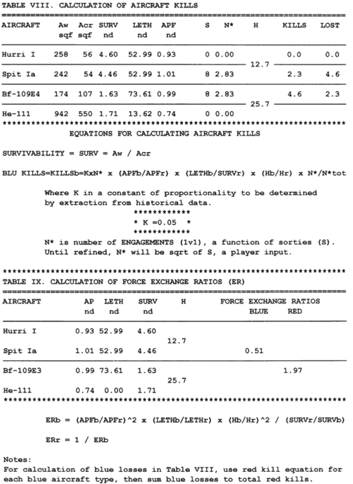
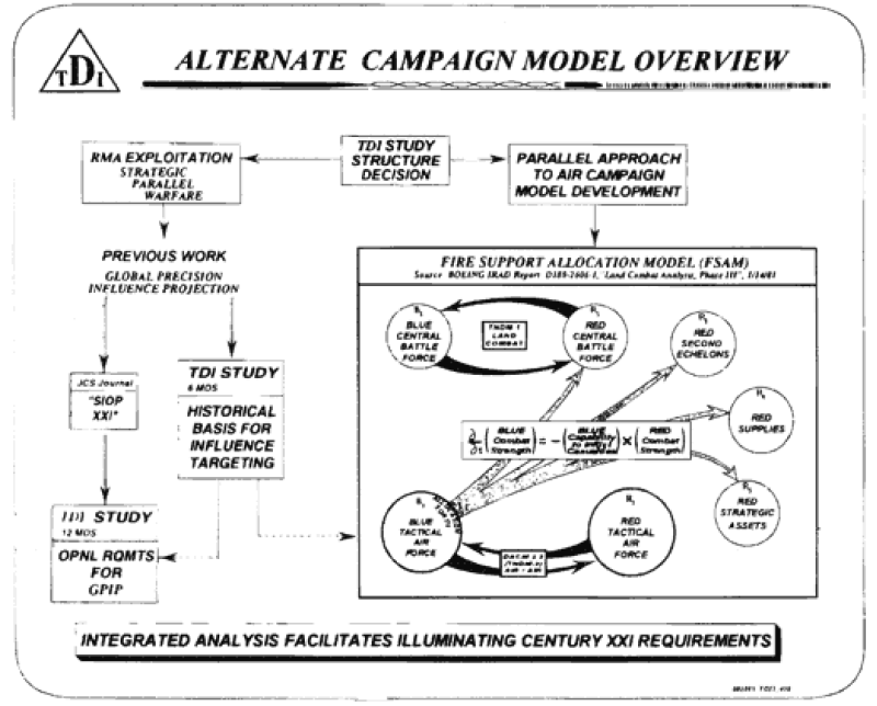
The Dupuy Air Campaign Model
by Col. Joseph A. Bulger, Jr., USAF, Ret.
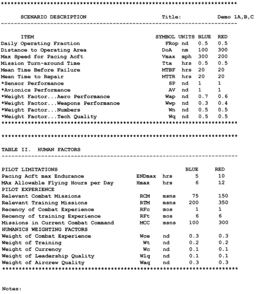
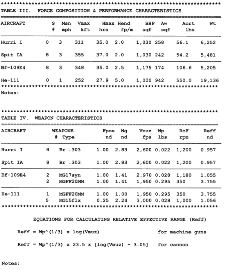
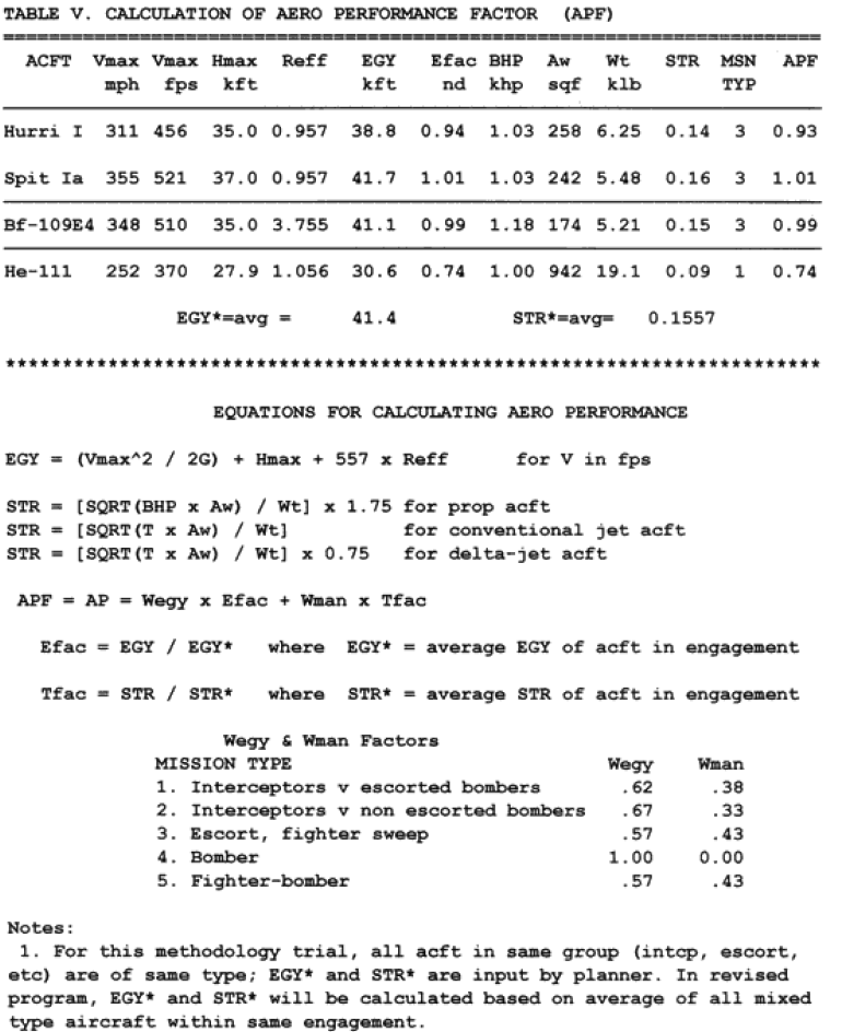
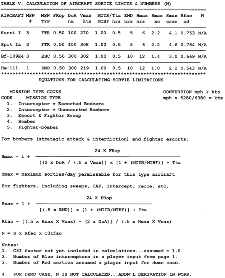
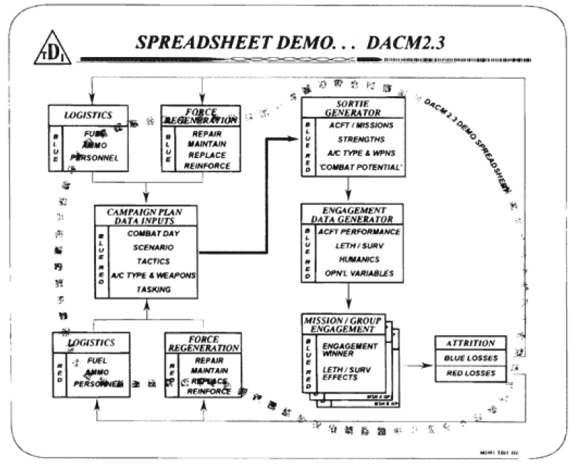
The Dupuy Institute, as part of the DACM [Dupuy Air Campaign Model], created a draft model in a spreadsheet format to show how such a model would calculate attrition. Below are the actual printouts of the “interim methodology demonstration,” which shows the types of inputs, outputs, and equations used for the DACM. The spreadsheet was created by Col. Bulger, while many of the formulae were the work of Robert Shaw.
Air Model Historical Data Study by Col. Joseph A. Bulger, Jr., USAF, Ret
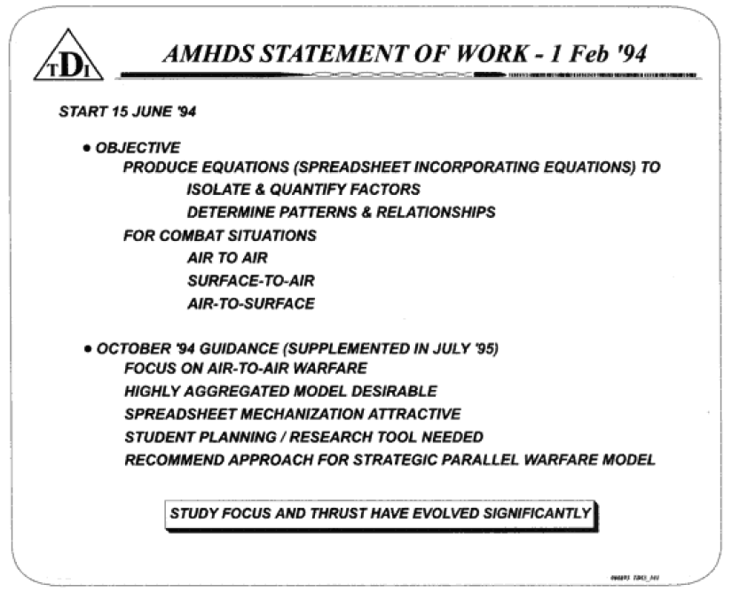
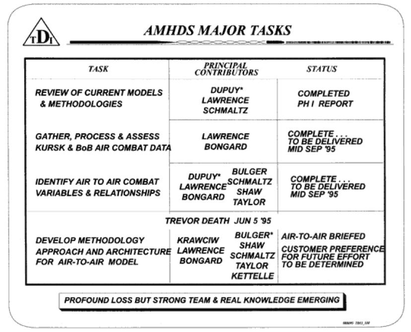
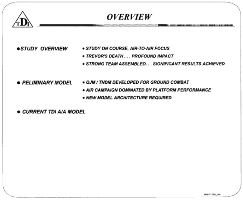
The Air Model Historical Study (AMHS) was designed to lead to the development of an air campaign model for use by the Air Command and Staff College (ACSC). This model, never completed, became known as the Dupuy Air Campaign Model (DACM). It was a team effort led by Trevor N. Dupuy and included the active participation of Lt. Col. Joseph Bulger, Gen. Nicholas Krawciw, Chris Lawrence, Dave Bongard, Robert Schmaltz, Robert Shaw, Dr. James Taylor, John Kettelle, Dr. George Daoust and Louis Zocchi, among others. After Dupuy’s death, I took over as the project manager.
At the first meeting of the team Dupuy assembled for the study, it became clear that this effort would be a serious challenge. In his own style, Dupuy was careful to provide essential guidance while, at the same time, cultivating a broad investigative approach to the unique demands of modeling for air combat. It would have been no surprise if the initial guidance established a focus on the analytical approach, level of aggregation, and overall philosophy of the QJM [Quantified Judgement Model] and TNDM [Tactical Numerical Deterministic Model]. It was clear that Trevor had no intention of steering the study into an air combat modeling methodology based directly on QJM/TNDM. To the contrary, he insisted on a rigorous derivation of the factors that would permit the final choice of model methodology.
At the time of Dupuy’s death in June 1995, the Air Model Historical Data Study had reached a point where a major decision was needed. The early months of the study had been devoted to developing a consensus among the TDI team members with respect to the factors that needed to be included in the model. The discussions tended to highlight three areas of particular interest—factors that had been included in models currently in use, the limitations of these models, and the need for new factors (and relationships) peculiar to the properties and dynamics of the air campaign. Team members formulated a family of relationships and factors, but the model architecture itself was not investigated beyond the surface considerations.
Despite substantial contributions from team members, including analytical demonstrations of selected factors and air combat relationships, no consensus had been achieved. On the contrary, there was a growing sense of need to abandon traditional modeling approaches in favor of a new application of the “Dupuy Method” based on a solid body of air combat data from WWII.
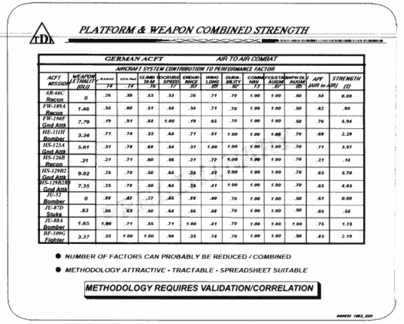
The Dupuy approach to modeling land combat relied heavily on the ratio of force strengths (largely determined by firepower as modified by other factors). After almost a year of investigations by the AMHDS team, it was beginning to appear that air combat differed in a fundamental way from ground combat. The essence of the difference is that in air combat, the outcome of the maneuver battle for platform position must be determined before the firepower relationships may be brought to bear on the battle outcome.
At the time of Dupuy’s death, it was apparent that if the study contract was to yield a meaningful product, an immediate choice of analysis thrust was required. Shortly prior to Dupuy’s death, I and other members of the TDI team recommended that we adopt the overall approach, level of aggregation, and analytical complexity that had characterized Dupuy’s models of land combat. We also agreed on the time-sequenced predominance of the maneuver phase of air combat. When I was asked to take the analytical lead for the contact in Dupuy’s absence, I was reasonably confident that there was overall agreement.
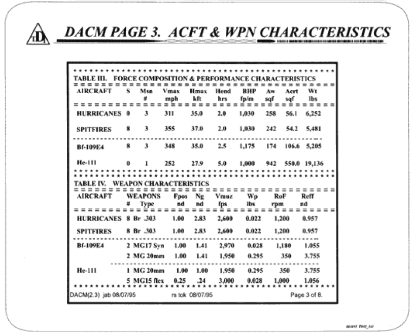
In view of the time available to prepare a deliverable product, it was decided to prepare a model using the air combat data we had been evaluating up to that point—June 1995. Fortunately, Robert Shaw had developed a set of preliminary analysis relationships that could be used in an initial assessment of the maneuver/firepower relationship. In view of the analytical, logistic, contractual, and time factors discussed, we decided to complete the contract effort based on the following analytical thrust:
The contract deliverable would be based on the maneuver/firepower analysis approach as currently formulated in Robert Shaw’s performance equations;
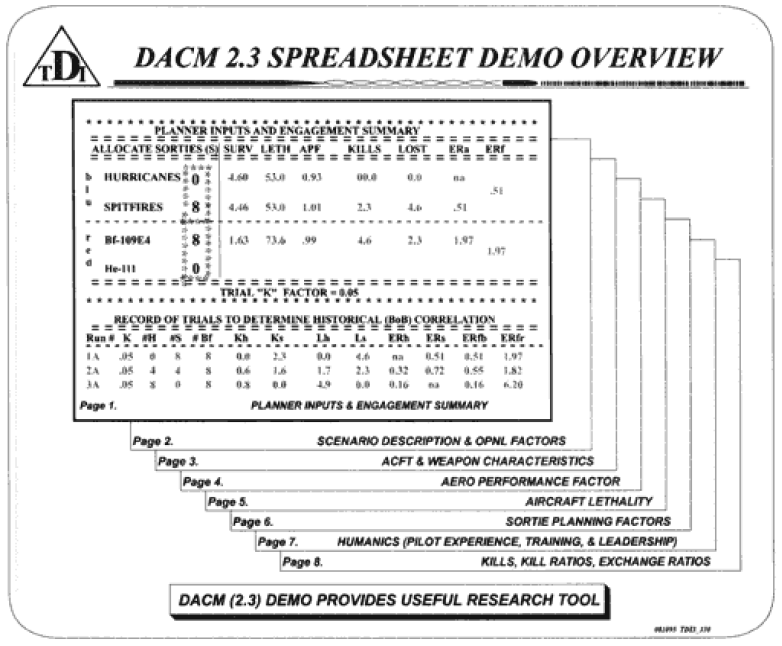
A spreadsheet formulation of outcomes for selected (Battle of Britain) engagements would be presented to the customer in August 1995;
To the extent practical, a working model would be provided to the customer with suggestions for further development.
During the following six weeks, the demonstration model was constructed. The model (programmed for a Lotus 1-2-3 style spreadsheet formulation) was developed, mechanized, and demonstrated to ACSC in August 1995. The final report was delivered in September of 1995.
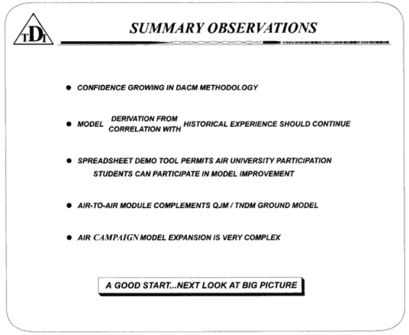
The working model demonstrated to ACSC in August 1995 suggests the following observations:
A substantial contribution to the understanding of air combat modeling has been achieved.
While relationships developed in the Dupuy Air Combat Model (DACM) are not fully mature, they are analytically significant.
The approach embodied in DACM derives its authenticity from the famous “Dupuy Method” thus ensuring its strong correlations with actual combat data.
Although demonstrated only for air combat in the Battle of Britain, the methodology is fully capable of incorporating modem technology contributions to sensor, command and control, and firepower performance.
The knowledge base, fundamental performance relationships, and methodology contributions embodied in DACM are worthy of further exploration. They await only the expression of interest and a relatively modest investment to extend the analysis methodology into modem air combat and the engagements anticipated for the 21st Century.
One final observation seems appropriate. The DACM demonstration provided to ACSC in August 1995 should not be dismissed as a perhaps interesting, but largely simplistic approach to air combat modeling. It is a significant contribution to the understanding of air combat relationships that will prevail in the 21st Century. The Dupuy Institute is convinced that further development of DACM makes eminent good sense. An exploitation of the maneuver and firepower relationships already demonstrated in DACM will provide a valid basis for modeling air combat with modern technology sensors, control mechanisms, and weapons. It is appropriate to include the Dupuy name in the title of this latest in a series of distinguished combat models. Trevor would be pleased.
Technology and the Human Factor in War by Trevor N. Dupuy
The Debate
It has become evident to many military theorists that technology has become increasingly important in war. In fact (even though many soldiers would not like to admit it) most such theorists believe that technology has actually reduced the significance of the human factor in war, In other words, the more advanced our military technology, these “technocrats” believe, the less we need to worry about the professional capability and competence of generals, admirals, soldiers, sailors, and airmen.
The technocrats believe that the results of the Kuwait, or Gulf, War of 1991 have confirmed their conviction. They cite the contribution to those results of the U.N. (mainly U.S.) command of the air, stealth aircraft, sophisticated guided missiles, and general electronic superiority, They believe that it was technology which simply made irrelevant the recent combat experience of the Iraqis in their long war with Iran.
Yet there are a few humanist military theorists who believe that the technocrats have totally misread the lessons of this century‘s wars! They agree that, while technology was important in the overwhelming U.N. victory, the principal reason for the tremendous margin of U.N. superiority was the better training, skill, and dedication of U.N. forces (again, mainly U.S.).
And so the debate rests. Both sides believe that the result of the Kuwait War favors their point of view, Nevertheless, an objective assessment of the literature in professional military journals, of doctrinal trends in the U.S. services, and (above all) of trends in the U.S. defense budget, suggest that the technocrats have stronger arguments than the humanists—or at least have been more convincing in presenting their arguments.
I suggest, however, that a completely impartial comparison of the Kuwait War results with those of other recent wars, and with some of the phenomena of World War II, shows that the humanists should not yet concede the debate.
I am a humanist, who is also convinced that technology is as important today in war as it ever was (and it has always been important), and that any national or military leader who neglects military technology does so to his peril and that of his country, But, paradoxically, perhaps to an extent even greater than ever before, the quality of military men is what wins wars and preserves nations.
To elevate the debate beyond generalities, and demonstrate convincingly that the human factor is at least as important as technology in war, I shall review eight instances in this past century when a military force has been successful because of the quality if its people, even though the other side was at least equal or superior in the technological sophistication of its weapons. The examples I shall use are:
Germany vs. the USSR in World War II
Germany vs. the West in World War II
Israel vs. Arabs in 1948, 1956, 1967, 1973 and 1982
The Vietnam War, 1965-1973
Britain vs. Argentina in the Falklands 1982
South Africans vs. Angolans and Cubans, 1987-88
The U.S. vs. Iraq, 1991
The demonstration will be based upon a marshaling of historical facts, then analyzing those facts by means of a little simple arithmetic.
Relative Combat Effectiveness Value (CEV)
The purpose of the arithmetic is to calculate relative combat effectiveness values (CEVs) of two opposing military forces. Let me digress to set up the arithmetic. Although some people who hail from south of the Mason-Dixon Line may be reluctant to accept the fact, statistics prove that the fighting quality of Northern soldiers and Southern soldiers was virtually equal in the American Civil War. (I invite those who might disagree to look at Livermore’s Numbers and Losses in the Civil War). That assumption of equality of the opposing troop quality in the Civil War enables me to assert that the successful side in every important battle in the Civil War was successful either because of numerical superiority or superior generalship. Three of Lee’s battles make the point:
Despite being outnumbered, Lee won at Antietam. (Though Antietam is sometimes claimed as a Union victory, Lee, the defender, held the battlefield; McClellan, the attacker, was repulsed.) The main reason for Lee’s success was that on a scale of leadership his generalship was worth 10, while McClellan was barely a 6.
Despite being outnumbered, Lee won at Chancellorsville because he was a 10 to Hooker’s 5.
Lee lost at Gettysburg mainly because he was outnumbered. Also relevant: Meade did not lose his nerve (like McClellan and Hooker) with generalship worth 8 to match Lee’s 8.
Let me use Antietam to show the arithmetic involved in those simple analyses of a rather complex subject:
The numerical strength of McClellan’s army was 89,000; Lee’s army was only 39,000 strong, but had the multiplier benefit of defensive posture. This enables us to calculate the theoretical combat power ratio of the Union Army to the Confederate Army as 1.4:1.0. In other words, with substantial preponderance of force, the Union Army should have been successful. (The combat power ratio of Confederates to Northerners, of course, was the reciprocal, or 0.71:1.04)
However, Lee held the battlefield, and a calculation of the actual combat power ratio of the two sides (based on accomplishment of mission, gaining or holding ground, and casualties) was a scant, but clear cut: 1.16:1.0 in favor of the Confederates. A ratio of the actual combat power ratio of the Confederate/Union armies (1.16) to their theoretical combat power (0.71) gives us a value of 1.63. This is the relative combat effectiveness of the Lee’s army to McClellan’s army on that bloody day. But, if we agree that the quality of the troops was the same, then the differential must essentially be in the quality of the opposing generals. Thus, Lee was a 10 to McClellan‘s 6.
The simple arithmetic equation[1] on which the above analysis was based is as follows:
CEV = (R/R)/(P/P)
When:
CEV is relative Combat Effectiveness Value
R/R is the actual combat power ratio
P/P is the theoretical combat power ratio.
At Antietam the equation was: 1.63 = 1.16/0.71.
We’ll be revisiting that equation in connection with each of our examples of the relative importance of technology and human factors.
Air Power and Technology
However, one more digression is required before we look at the examples. Air power was important in all eight of the 20th Century examples listed above. Offhand it would seem that the exercise of air superiority by one side or the other is a manifestation of technological superiority. Nevertheless, there are a few examples of an air force gaining air superiority with equivalent, or even inferior aircraft (in quality or numbers) because of the skill of the pilots.
However, the instances of such a phenomenon are rare. It can be safely asserted that, in the examples used in the following comparisons, the ability to exercise air superiority was essentially a technological superiority (even though in some instances it was magnified by human quality superiority). The one possible exception might be the Eastern Front in World War II, where a slight German technological superiority in the air was offset by larger numbers of Soviet aircraft, thanks in large part to Lend-Lease assistance from the United States and Great Britain.
The Battle of Kursk, 5-18 July, 1943
Following the surrender of the German Sixth Army at Stalingrad, on 2 February, 1943, the Soviets mounted a major winter offensive in south-central Russia and Ukraine which reconquered large areas which the Germans had overrun in 1941 and 1942. A brilliant counteroffensive by German Marshal Erich von Manstein‘s Army Group South halted the Soviet advance, and recaptured the city of Kharkov in mid-March. The end of these operations left the Soviets holding a huge bulge, or salient, jutting westward around the Russian city of Kursk, northwest of Kharkov.
The Germans promptly prepared a new offensive to cut off the Kursk salient, The Soviets energetically built field fortifications to defend the salient against expected German attacks. The German plan was for simultaneous offensives against the northern and southern shoulders of the base of the Kursk salient, Field Marshal Gunther von K1uge’s Army Group Center, would drive south from the vicinity of Orel, while Manstein’s Army Group South pushed north from the Kharkov area, The offensive was originally scheduled for early May, but postponements by Hitler, to equip his forces with new tanks, delayed the operation for two months, The Soviets took advantage of the delays to further improve their already formidable defenses.
The German attacks finally began on 5 July. In the north General Walter Model’s German Ninth Army was soon halted by Marshal Konstantin Rokossovski’s Army Group Center. In the south, however, German General Hermann Hoth’s Fourth Panzer Army and a provisional army commanded by General Werner Kempf, were more successful against the Voronezh Army Group of General Nikolai Vatutin. For more than a week the XLVIII Panzer Corps advanced steadily toward Oboyan and Kursk through the most heavily fortified region since the Western Front of 1918. While the Germans suffered severe casualties, they inflicted horrible losses on the defending Soviets. Advancing similarly further east, the II SS Panzer Corps, in the largest tank battle in history, repulsed a vigorous Soviet armored counterattack at Prokhorovka on July 12-13, but was unable to continue to advance.
The principal reason for the German halt was the fact that the Soviets had thrown into the battle General Ivan Konev’s Steppe Army Group, which had been in reserve. The exhausted, heavily outnumbered Germans had no comparable reserves to commit to reinvigorate their offensive.
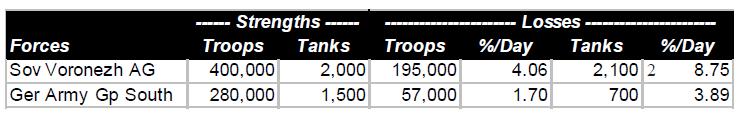
A comparison of forces and losses of the Soviet Voronezh Army Group and German Army Group South on the south face of the Kursk Salient is shown below. The strengths are averages over the 12 days of the battle, taking into consideration initial strengths, losses, and reinforcements.
A comparison of the casualty tradeoff can be found by dividing Soviet casualties by German strength, and German losses by Soviet strength. On that basis, 100 Germans inflicted 5.8 casualties per day on the Soviets, while 100 Soviets inflicted 1.2 casualties per day on the Germans, a tradeoff of 4.9 to 1.0
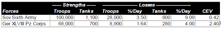
The statistics for the 8-day offensive of the German XLVIII Panzer Corps toward Oboyan are shown below. Also shown is the relative combat effectiveness value (CEV) of Germans and Soviets, as calculated by the TNDM. As was the case for the Battle of Antietam, this is derived from a mathematical comparison of the theoretical combat power ratio of the two forces (simply considering numbers and weapons characteristics), and the actual combat power ratios reflected by the battle results:
The calculated CEVs suggest that 100 German troops were the combat equivalent of 240 Soviet troops, comparably equipped. The casualty tradeoff in this battle shows that 100 Germans inflicted 5.15 casualties per day on the Soviets, while 100 Soviets inflicted 1.11 casualties per day on the Germans, a tradeoff of4.64. It is a rule of thumb that the casualty tradeoff is usually about the square of the CEV.
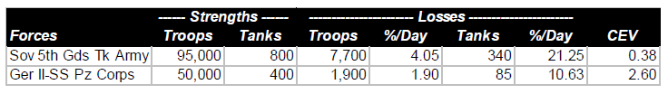
A similar comparison can be made of the two-day battle of Prokhorovka. Soviet accounts of that battle have claimed this as a great victory by the Soviet Fifth Guards Tank Army over the German II SS Panzer Corps. In fact, since the German advance was halted, the outcome was close to a draw, but with the advantage clearly in favor of the Germans.
The casualty tradeoff shows that 100 Germans inflicted 7.7 casualties per on the Soviets, while 100 Soviets inflicted 1.0 casualties per day on the Germans, for a tradeoff value of 7.7.
When the German offensive began, they had a slight degree of local air superiority. This was soon reversed by German and Soviet shifts of air elements, and during most of the offensive, the Soviets had a slender margin of air superiority. In terms of technology, the Germans probably had a slight overall advantage. However, the Soviets had more tanks and, furthermore, their T-34 was superior to any tank the Germans had available at the time. The CEV calculations demonstrate that the Germans had a great qualitative superiority over the Russians, despite near-equality in technology, and despite Soviet air superiority. The Germans lost the battle, but only because they were overwhelmed by Soviet numbers.
German Performance, Western Europe, 1943-1945
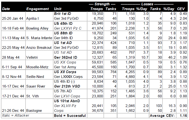
Beginning with operations between Salerno and Naples in September, 1943, through engagements in the closing days of the Battle of the Bulge in January, 1945, the pattern of German performance against the Western Allies was consistent. Some German units were better than others, and a few Allied units were as good as the best of the Germans. But on the average, German performance, as measured by CEV and casualty tradeoff, was better than the Western allies by a CEV factor averaging about 1.2, and a casualty tradeoff factor averaging about 1.5. Listed below are ten engagements from Italy and Northwest Europe during that 1944.
Technologically, German forces and those of the Western Allies were comparable. The Germans had a higher proportion of armored combat vehicles, and their best tanks were considerably better than the best American and British tanks, but the advantages were at least offset by the greater quantity of Allied armor, and greater sophistication of much of the Allied equipment. The Allies were increasingly able to achieve and maintain air superiority during this period of slightly less than two years.
The combination of vast superiority in numbers of troops and equipment, and in increasing Allied air superiority, enabled the Allies to fight their way slowly up the Italian boot, and between June and December, 1944, to drive from the Normandy beaches to the frontier of Germany. Yet the presence or absence of Allied air support made little difference in terms of either CEVs or casualty tradeoff values. Despite the defeats inflicted on them by the numerically superior Allies during the latter part of 1944, in December the Germans were able to mount a major offensive that nearly destroyed an American army corps, and threatened to drive at least a portion of the Allied armies into the sea.
Clearly, in their battles against the Soviets and the Western Allies, the Germans demonstrated that quality of combat troops was able consistently to overcome Allied technological and air superiority. It was Allied numbers, not technology, that defeated the quantitatively superior Germans.
The Six-Day War, 1967
The remarkable Israeli victories over far more numerous Arab opponents—Egyptian, Jordanian, and Syrian—in June, 1967 revealed an Israeli combat superiority that had not been suspected in the United States, the Soviet Union or Western Europe. This superiority was equally awesome on the ground as in the air. (By beginning the war with a surprise attack which almost wiped out the Egyptian Air Force, the Israelis avoided a serious contest with the one Arab air force large enough, and possibly effective enough, to challenge them.) The results of the three brief campaigns are summarized in the table below:
It should be noted that some Israelis who fought against the Egyptians and Jordanians also fought against the Syrians. Thus, the overall Arab numerical superiority was greater than would be suggested by adding the above strength figures, and was approximately 328,000 to 200,000.
It should also be noted that the technological sophistication of the Israeli and Arab ground forces was comparable. The only significant technological advantage of the Israelis was their unchallenged command of the air. (In terms of battle outcomes, it was irrelevant how they had achieved air superiority.) In fact this was a very significant advantage, the full import of which would not be realized until the next Arab-Israeli war.
The results of the Six Day War do not provide an unequivocal basis for determining the relative importance of human factors and technological superiority (as evidenced in the air). Clearly a major factor in the Israeli victories was the superior performance of their ground forces due mainly to human factors. At least as important in those victories was Israeli command of the air, in which both technology and human factors both played a part.
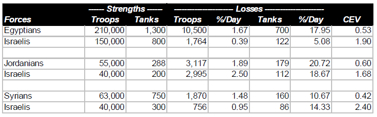
The October War, 1973
A better basis for comparing the relative importance of human factors and technology is provided by the results of the October War of 1973 (known to Arabs as the War of Ramadan, and to Israelis as the Yom Kippur War). In this war the Israeli unquestioned superiority in the air was largely offset by the Arabs possession of highly sophisticated Soviet air defense weapons.
One important lesson of this war was a reassessment of Israeli contempt for the fighting quality of Arab ground forces (which had stemmed from the ease with which they had won their ground victories in 1967). When Arab ground troops were protected from Israeli air superiority by their air defense weapons, they fought well and bravely, demonstrating that Israeli control of the air had been even more significant in 1967 than anyone had then recognized.
It should be noted that the total Arab (and Israeli) forces are those shown in the first two comparisons, above. A Jordanian brigade and two Iraqi divisions formed relatively minor elements of the forces under Syrian command (although their presence on the ground was significant in enabling the Syrians to maintain a defensive line when the Israelis threatened a breakthrough around 20 October). For the comparison of Jordanians and Iraqis the total strength is the total of the forces in the battles (two each) on which these comparisons are based.
One other thing to note is how the Israelis, possibly unconsciously, confirmed that validity of their CEVs with respect to Egyptians and Syrians by the numerical strengths of their deployments to the two fronts. Since the war ended up in a virtual stalemate on both fronts, the overall strength figures suggest rough equivalence of combat capability.
The CEV values shown in the above table are very significant in relation to the debate about human factors and technology, There was little if anything to choose between the technological sophistication of the two sides. The Arabs had more tanks than the Israelis, but (as Israeli General Avraham Adan once told the author) there was little difference in the quality of the tanks. The Israelis again had command of the air, but this was neutralized immediately over the battlefields by the Soviet air defense equipment effectively manned by the Arabs. Thus, while technology was of the utmost importance to both sides, enabling each side to prevent the enemy from gaining a significant advantage, the true determinant of battlefield outcomes was the fighting quality of the troops, And, while the Arabs fought bravely, the Israelis fought much more effectively. Human factors made the difference.
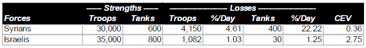
Israeli Invasion of Lebanon, 1982
In terms of the debate about the relative importance of human factors and technology, there are two significant aspects to this small war, in which Syrians forces and PLO guerrillas were the Arab participants. In the first place, the Israelis showed that their air technology was superior to the Syrian air defense technology, As a result, they regained complete control of the skies over the battlefields. Secondly, it provides an opportunity to include a highly relevant quotation.
The statistical comparison shows the results of the two major battles fought between Syrians and Israelis:
In assessing the above statistics, a quotation from the Israeli Chief of Staff, General Rafael Eytan, is relevant.
In late 1982 a group of retired American generals visited Israel and the battlefields in Lebanon. Just before they left for home, they had a meeting with General Eytan. One of the American generals asked Eytan the following question: “Since the Syrians were equipped with Soviet weapons, and your troops were equipped with American (or American-type) weapons, isn’t the overwhelming Israeli victory an indication of the superiority of American weapons technology over Soviet weapons technology?”
Eytan’s reply was classic: “If we had had their weapons, and they had had ours, the result would have been absolutely the same.”
One need not question how the Israeli Chief of Staff assessed the relative importance of the technology and human factors.
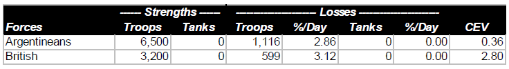
Falkland Islands War, 1982
It is difficult to get reliable data on the Falkland Islands War of 1982. Furthermore, the author of this article had not undertaken the kind of detailed analysis of such data as is available. However, it is evident from the information that is available about that war that its results were consistent with those of the other examples examined in this article.
The total strength of Argentine forces in the Falklands at the time of the British counter-invasion was slightly more than 13,000. The British appear to have landed close to 6,400 troops, although it may have been fewer. In any event, it is evident that not more than 50% of the total forces available to both sides were actually committed to battle. The Argentine surrender came 27 days after the British landings, but there were probably no more than six days of actual combat. During these battles the British performed admirably, the Argentinians performed miserably. (Save for their Air Force, which seems to have fought with considerable gallantry and effectiveness, at the extreme limit of its range.) The British CEV in ground combat was probably between 2.5 and 4.0. The statistics were at least close to those presented below:
It is evident from published sources that the British had no technological advantage over the Argentinians; thus the one-sided results of the ground battles were due entirely to British skill (derived from training and doctrine) and determination.
South African Operations in Angola, 1987-1988
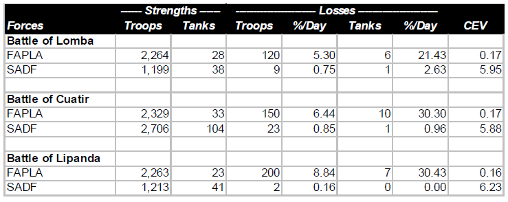
Neither the political reasons for, nor political results of, the South African military interventions in Angola in the 1970s, and again in the late 1980s, need concern us in our consideration of the relative significance of technology and of human factors. The combat results of those interventions, particularly in 1987-1988 are, however, very relevant.
The operations between elements of the South African Defense Force (SADF) and forces of the Popular Movement for the Liberation of Angola (FAPLA) took place in southeast Angola, generally in the region east of the city of Cuito-Cuanavale. Operating with the SADF units were a few small units of Jonas Savimbi’s National Union for the Total Independence of Angola (UNITA). To provide air support to the SADF and UNITA ground forces, it would have been necessary for the South Africans to establish air bases either in Botswana, Southwest Africa (Namibia), or in Angola itself. For reasons that were largely political, they decided not to do that, and thus operated under conditions of FAPLA air supremacy. This led them, despite terrain generally unsuited for armored warfare, to use a high proportion of armored vehicles (mostly light armored cars) to provide their ground troops with some protection from air attack.
Summarized below are the results of three battles east of Cuito-Cuanavale in late 1987 and early 1988. Included with FAPLA forces are a few Cubans (mostly in armored units); included with the SADF forces are a few UNITA units (all infantry).
FAPLA had complete command of air, and substantial numbers of MiG-21 and MiG-23 sorties were flown against the South Africans in all of these battles. This technological superiority was probably partly offset by greater South African EW (electronic warfare) capability. The ability of the South Africans to operate effectively despite hostile air superiority was reminiscent of that of the Germans in World War II. It was a further demonstration that, no matter how important technology may be, the fighting quality of the troops is even more important.
The tank figures include armored cars. In the first of the three battles considered, FAPLA had by far the more powerful and more numerous medium tanks (20 to 0). In the other two, SADF had a slight or significant advantage in medium tank numbers and quality. But it didn’t seem to make much difference in the outcomes.
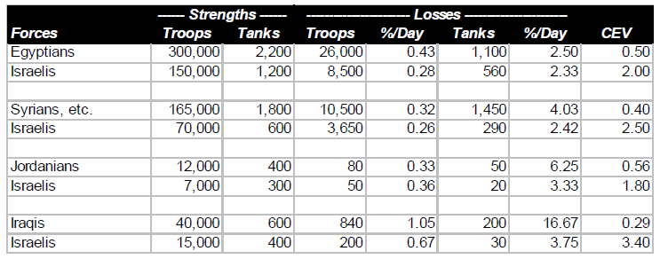
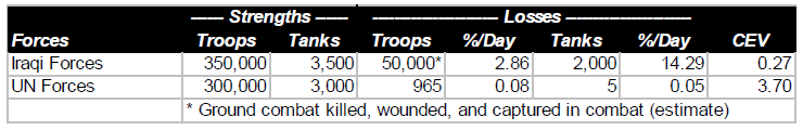
Kuwait War, 1991
The previous seven examples permit us to examine the results of Kuwait (or Second Gulf) War with more objectivity than might otherwise have possible. First, let’s look at the statistics. Note that the comparison shown below is for four days of ground combat, February 24-28, and shows only operations of U.S. forces against the Iraqis.
There can be no question that the single most important contribution to the overwhelming victory of U.S. and other U.N. forces was the air war that preceded, and accompanied, the ground operations. But two comments are in order. The air war alone could not have forced the Iraqis to surrender. On the other hand, it is evident that, even without the air war, U.S. forces would have readily overwhelmed the Iraqis, probably in more than four days, and with more than 285 casualties. But the outcome would have been hardly less one-sided.
The Vietnam War, 1965-1973
It is impossible to make the kind of mathematical analysis for the Vietnam War as has been done in the examples considered above. The reason is that we don’t have any good data on the Vietcong—North Vietnamese forces,
However, such quantitative analysis really isn’t necessary There can be no doubt that one of the opponents was a superpower, the most technologically advanced nation on earth, while the other side was what Lyndon Johnson called a “raggedy-ass little nation,” a typical representative of “the third world.“
Furthermore, even if we were able to make the analyses, they would very possibly be misinterpreted. It can be argued (possibly with some exaggeration) that the Americans won all of the battles. The detailed engagement analyses could only confirm this fact. Yet it is unquestionable that the United States, despite airpower and all other manifestations of technological superiority, lost the war. The human factor—as represented by the quality of American political (and to a lesser extent military) leadership on the one side, and the determination of the North Vietnamese on the other side—was responsible for this defeat.
Conclusion
In a recent article in the Armed Forces Journal International Col. Philip S. Neilinger, USAF, wrote: “Military operations are extremely difficult, if not impossible, for the side that doesn’t control the sky.” From what we have seen, this is only partly true. And while there can be no question that operations will always be difficult to some extent for the side that doesn’t control the sky, the degree of difficulty depends to a great degree upon the training and determination of the troops.
What we have seen above also enables us to view with a better perspective Colonel Neilinger’s subsequent quote from British Field Marshal Montgomery: “If we lose the war in the air, we lose the war and we lose it quickly.” That statement was true for Montgomery, and for the Allied troops in World War II. But it was emphatically not true for the Germans.
The examples we have seen from relatively recent wars, therefore, enable us to establish priorities on assuring readiness for war. It is without question important for us to equip our troops with weapons and other materiel which can match, or come close to matching, the technological quality of the opposition’s materiel. We must realize that we cannot—as some people seem to think—buy good forces, by technology alone. Even more important is to assure the fighting quality of the troops. That must be, by far, our first priority in peacetime budgets and in peacetime military activities of all sorts.
NOTES
[1] This calculation is automatic in analyses of historical battles by the Tactical Numerical Deterministic Model (TNDM).
[2] The initial tank strength of the Voronezh Army Group was about 1,100 tanks. About 3,000 additional Soviet tanks joined the battle between 6 and 12 July. At the end of the battle there were about 1,800 Soviet tanks operational in the battle area; at the same time there were about 1,000 German tanks still operational.
[3] The relative combat effectiveness value of each force is calculated in comparison to 1.0. Thus the CEV of the Germans is 2.40:1.0, while that of the Soviets is 0.42: 1.0. The opposing CEVs are always the reciprocals of each other.


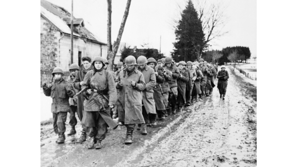
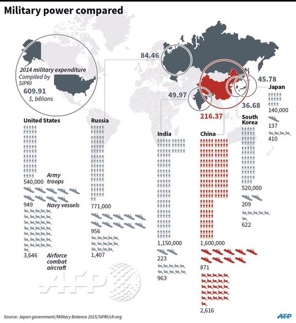 [This article was originally posted on 11 October 2016]