The Military Operations Research Society (MORS) publishes a periodical journal called the Phalanx. In the December 2018 issue was an article that referenced one of our blog posts. This took us by surprise. We only found out about thanks to one of the viewers of this blog. We are not members of MORS. The article is paywalled and cannot be easily accessed if you are not a member.
It is titled “Perspectives on Combat Modeling” (page 28) and is written by Jonathan K. Alt, U.S. Army TRADOC Analysis Center, Monterey, CA.; Christopher Morey, PhD, Training and Doctrine Command Analysis Center, Ft. Leavenworth, Kansas; and Larry Larimer, Training and Doctrine Command Analysis Center, White Sands, New Mexico. I am not familiar with any of these three gentlemen.
The blog post that appears to be generating this article is this one:
Simply by coincidence, Shawn Woodford recently re-posted this in January. It was originally published on 10 April 2017 and was written by Shawn.
The opening two sentences of the article in the Phalanx reads:
Periodically, within the Department of Defense (DoD) analytic community, questions will arise regarding the validity of the combat models and simulations used to support analysis. Many attempts (sic) to resurrect the argument that models, simulations, and wargames “are built on the thin foundation of empirical knowledge about the phenomenon of combat.” (Woodford, 2017).
It is nice to be acknowledged, although it this case, it appears that we are being acknowledged because they disagree with what we are saying.
Probably the word that gets my attention is “resurrect.” It is an interesting word, that implies that this is an old argument that has somehow or the other been put to bed. Granted it is an old argument. On the other hand, it has not been put to bed. If a problem has been identified and not corrected, then it is still a problem. Age has nothing to do with it.
On the other hand, maybe they are using the word “resurrect” because recent developments in modeling and validation have changed the environment significantly enough that these arguments no longer apply. If so, I would be interested in what those changes are. The last time I checked, the modeling and simulation industry was using many of the same models they had used for decades. In some cases, were going back to using simpler hex-games for their modeling and wargaming efforts. We have blogged a couple of times about these efforts. So, in the world of modeling, unless there have been earthshaking and universal changes made in the last five years that have completely revamped the landscape….then the decades old problems still apply to the decades old models and simulations.
More to come (this is the first of at least 7 posts on this subject).
Source: David A. Shlapak and Michael Johnson. Reinforcing Deterrence on NATO’s Eastern Flank: Wargaming the Defense of the Baltics. Santa Monica, CA: RAND Corporation, 2016.
[UPDATE] We had several readers recommend games they have used or would be suitable for simulating Multi-Domain Battle and Operations (MDB/MDO) concepts. These include several classic campaign-level board wargames:
Chris Lawrence recently looked at C-WAM and found that it uses a lot of traditional board wargaming elements, including methodologies for determining combat results, casualties, and breakpoints that have been found unable to replicate real-world outcomes (aka “The Base of Sand” problem).
What other wargames, models, and simulations are there being used out there? Are there any commercial wargames incorporating MDB/MDO elements into their gameplay? What methodologies are being used to portray MDB/MDO effects?
A great deal of importance has been placed on the knowledge derived from these activities. As the U.S. Army Training and Doctrine Command recently stated,
Concept analysis informed by joint and multinational learning events…will yield the capabilities required of multi-domain battle. Resulting doctrine, organization, training, materiel, leadership, personnel and facilities solutions will increase the capacity and capability of the future force while incorporating new formations and organizations.
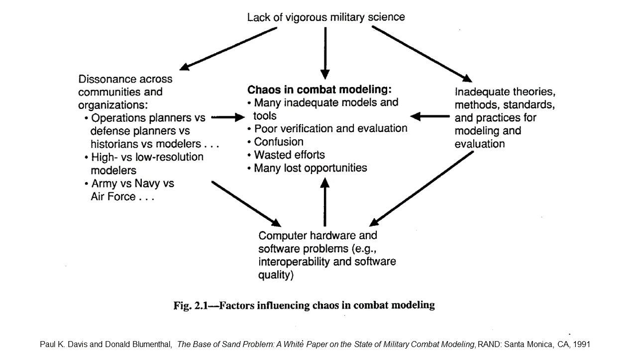
There is, however, a problem afflicting the Defense Department’s wargames, of which the military operations research and models and simulations communities have long been aware, but have been slow to address: their models are built on a thin foundation of empirical knowledge about the phenomenon of combat. None have proven the ability to replicate real-world battle experience. This is known as the “base of sand” problem.
A Brief History of The Base of Sand
All combat models and simulations are abstracted theories of how combat works. Combat modeling in the United States began in the early 1950s as an extension of military operations research that began during World War II. Early model designers did not have large base of empirical combat data from which to derive their models. Although a start had been made during World War II and the Korean War to collect real-world battlefield data from observation and military unit records, an effort that provided useful initial insights, no systematic effort has ever been made to identify and assemble such information. In the absence of extensive empirical combat data, model designers turned instead to concepts of combat drawn from official military doctrine (usually of uncertain provenance), subject matter expertise, historians and theorists, the physical sciences, or their own best guesses.
As the U.S. government’s interest in scientific management methods blossomed in the late 1950s and 1960s, the Defense Department’s support for operations research and use of combat modeling in planning and analysis grew as well. By the early 1970s, it became evident that basic research on combat had not kept pace. A survey of existing combat models by Gary Shubik and Martin Brewer for RAND in 1972 concluded that
Basic research and knowledge is lacking. The majority of the MSGs [models, simulations and games] sampled are living off a very slender intellectual investment in fundamental knowledge…. [T]he need for basic research is so critical that if no other funding were available we would favor a plan to reduce by a significant proportion all current expenditures for MSGs and to use the saving for basic research.
The [Defense Department]is becoming critically dependent on combat models (including simulations and war games)—even more dependent than in the past. There is considerable activity to improve model interoperability and capabilities for distributed war gaming. In contrast to this interest in model-related technology, there has been far too little interest in the substance of the models and the validity of the lessons learned from using them. In our view, the DoD does not appreciate that in many cases the models are built on a base of sand…
[T]he DoD’s approach in developing and using combat models, including simulations and war games, is fatally flawed—so flawed that it cannot be corrected with anything less than structural changes in management and concept. [Original emphasis]
As a remedy, the authors recommended that the Defense Department create an office to stimulate a national military science program. This Office of Military Science would promote and sponsor basic research on war and warfare while still relying on the military services and other agencies for most research and analysis.
Davis and Blumenthal initially drafted their white paper before the 1991 Gulf War, but the performance of the Defense Department’s models and simulations in that conflict underscored the very problems they described. Defense Department wargames during initial planning for the conflict reportedly predicted tens of thousands of U.S. combat casualties. These simulations were said to have led to major changes in U.S. Central Command’s operational plan. When the casualty estimates leaked, they caused great public consternation and inevitable Congressional hearings.
The Defense Department’s current generation of models and simulations harbor the same weaknesses as the ones in use in the 1990s. Some are new iterations of old models with updated graphics and code, but using the same theoretical assumptions about combat. In most cases, no one other than the designers knows exactly what data and concepts the models are based upon. This practice is known in the technology world as black boxing. While black boxing may be an essential business practice in the competitive world of government consulting, it makes independently evaluating the validity of combat models and simulations nearly impossible. This should be of major concern because many models and simulations in use today contain known flaws.
Others, such as the Joint Conflict And Tactical Simulation (JCATS), MAGTF Tactical Warfare System (MTWS), and Warfighters’ Simulation (WARSIM) adjudicate ground combat using probability of hit/probability of kill (pH/pK) algorithms. Corps Battle Simulation (CBS) uses pH/pK for direct fire attrition and a modified version of Lanchester for indirect fire. While these probabilities are developed from real-world weapon system proving ground data, their application in the models is combined with inputs from subjective sources, such as outputs from other combat models, which are likely not based on real-world data. Multiplying an empirically-derived figure by a judgement-based coefficient results in a judgement-based estimate, which might be accurate or it might not. No one really knows.
This state of affairs seems remarkable given the enormous stakes that are being placed on the output of the Defense Department’s modeling and simulation activities. After decades of neglect, remedying this would require a dedicated commitment to sustained basic research on the military science of combat and warfare, with no promise of a tangible short-term return on investment. Yet, as Biddle pointed out, “With so much at stake, we surely must do better.”
[NOTE: The attrition methodologies used in CBS and WARSIM have been corrected since this post was originally published per comments provided by their developers.]
There are three versions of force ratio versus casualty exchange ratio rules, such as the three-to-one rule (3-to-1 rule), as it applies to casualties. The earliest version of the rule as it relates to casualties that we have been able to find comes from the 1958 version of the U.S. Army Maneuver Control manual, which states: “When opposing forces are in contact, casualties are assessed in inverse ratio to combat power. For friendly forces advancing with a combat power superiority of 5 to 1, losses to friendly forces will be about 1/5 of those suffered by the opposing force.”[1]
The RAND version of the rule (1992) states that: “the famous ‘3:1 rule ’, according to which the attacker and defender suffer equal fractional loss rates at a 3:1 force ratio the battle is in mixed terrain and the defender enjoys ‘prepared ’defenses…” [2]
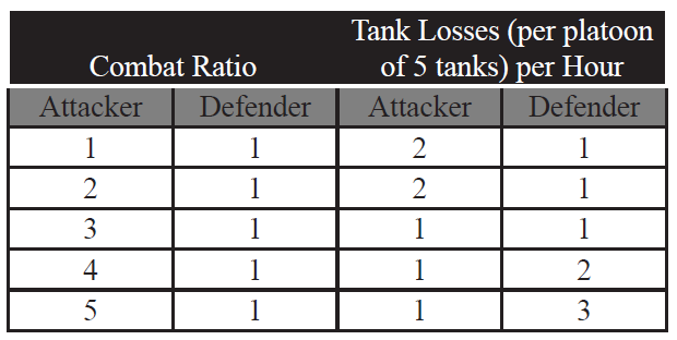
Finally, there is a version of the rule that dates from the 1967 Maneuver Control manual that only applies to armor that shows:
As the RAND construct also applies to equipment losses, then this formulation is directly comparable to the RAND construct.
Therefore, we have three basic versions of the 3-to-1 rule as it applies to casualties and/or equipment losses. First, there is a rule that states that there is an even fractional loss ratio at 3-to-1 (the RAND version), Second, there is a rule that states that at 3-to-1, the attacker will suffer one-third the losses of the defender. And third, there is a rule that states that at 3-to-1, the attacker and defender will suffer the same losses as the defender. Furthermore, these examples are highly contradictory, with either the attacker suffering three times the losses of the defender, the attacker suffering the same losses as the defender, or the attacker suffering 1/3 the losses of the defender.
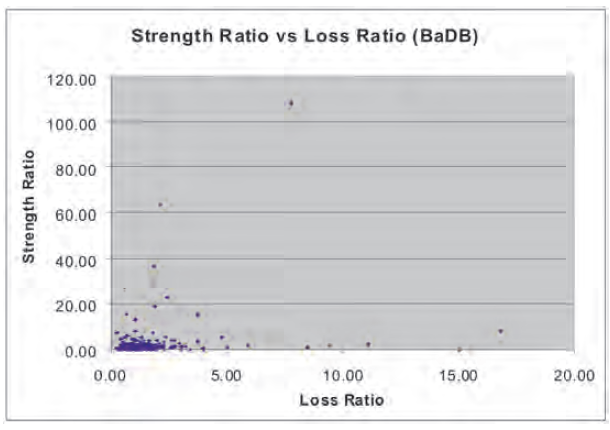
Therefore, what we will examine here is the relationship between force ratios and exchange ratios. In this case, we will first look at The Dupuy Institute’s Battles Database (BaDB), which covers 243 battles from 1600 to 1900. We will chart on the y-axis the force ratio as measured by a count of the number of people on each side of the forces deployed for battle. The force ratio is the number of attackers divided by the number of defenders. On the x-axis is the exchange ratio, which is a measured by a count of the number of people on each side who were killed, wounded, missing or captured during that battle. It does not include disease and non-battle injuries. Again, it is calculated by dividing the total attacker casualties by the total defender casualties. The results are provided below:
As can be seen, there are a few extreme outliers among these 243 data points. The most extreme, the Battle of Tippennuir (l Sep 1644), in which an English Royalist force under Montrose routed an attack by Scottish Covenanter militia, causing about 3,000 casualties to the Scots in exchange for a single (allegedly self-inflicted) casualty to the Royalists, was removed from the chart. This 3,000-to-1 loss ratio was deemed too great an outlier to be of value in the analysis.
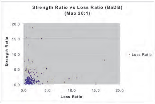
As it is, the vast majority of cases are clumped down into the corner of the graph with only a few scattered data points outside of that clumping. If one did try to establish some form of curvilinear relationship, one would end up drawing a hyperbola. It is worthwhile to look inside that clump of data to see what it shows. Therefore, we will look at the graph truncated so as to show only force ratios at or below 20-to-1 and exchange rations at or below 20-to-1.
Again, the data remains clustered in one corner with the outlying data points again pointing to a hyperbola as the only real fitting curvilinear relationship. Let’s look at little deeper into the data by truncating the data on 6-to-1 for both force ratios and exchange ratios. As can be seen, if the RAND version of the 3-to-1 rule is correct, then the data should show at 3-to-1 force ratio a 3-to-1 casualty exchange ratio. There is only one data point that comes close to this out of the 243 points we examined.
If the FM 105-5 version of the rule as it applies to armor is correct, then the data should show that at 3-to-1 force ratio there is a 1-to-1 casualty exchange ratio, at a 4-to-1 force ratio a 1-to-2 casualty exchange ratio, and at a 5-to-1 force ratio a 1-to-3 casualty exchange ratio. Of course, there is no armor in these pre-WW I engagements, but again no such exchange pattern does appear.
If the 1958 version of the FM 105-5 rule as it applies to casualties is correct, then the data should show that at a 3-to-1 force ratio there is 0.33-to-1 casualty exchange ratio, at a 4-to-1 force ratio a .25-to-1 casualty exchange ratio, and at a 5-to-1 force ratio a 0.20-to-5 casualty exchange ratio. As can be seen, there is not much indication of this pattern, or for that matter any of the three patterns.
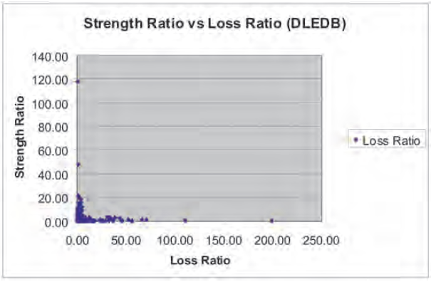
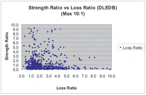
Still, such a construct may not be relevant to data before 1900. For example, Lanchester claimed in 1914 in Chapter V, “The Principal of Concentration,” of his book Aircraft in Warfare, that there is greater advantage to be gained in modern warfare from concentration of fire.[3] Therefore, we will tap our more modern Division-Level Engagement Database (DLEDB) of 675 engagements, of which 628 have force ratios and exchange ratios calculated for them. These 628 cases are then placed on a scattergram to see if we can detect any similar patterns.
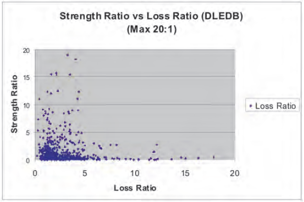
Even though this data covers from 1904 to 1991, with the vast majority of the data coming from engagements after 1940, one again sees the same pattern as with the data from 1600-1900. If there is a curvilinear relationship, it is again a hyperbola. As before, it is useful to look into the mass of data clustered into the corner by truncating the force and exchange ratios at 20-to-1. This produces the following:
Again, one sees the data clustered in the corner, with any curvilinear relationship again being a hyperbola. A look at the data further truncated to a 10-to-1 force or exchange ratio does not yield anything more revealing.
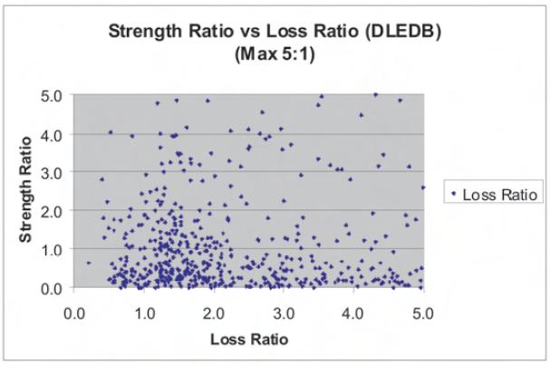
And, if this data is truncated to show only 5-to-1 force ratio and exchange ratios, one again sees:
Again, this data appears to be mostly just noise, with no clear patterns here that support any of the three constructs. In the case of the RAND version of the 3-to-1 rule, there is again only one data point (out of 628) that is anywhere close to the crossover point (even fractional exchange rate) that RAND postulates. In fact, it almost looks like the data conspires to make sure it leaves a noticeable “hole” at that point. The other postulated versions of the 3-to-1 rules are also given no support in these charts.
While we can attempt to torture the data to find a better fit, or can try to argue that the patterns are obscured by various factors that have not been considered, we do not believe that such a clear pattern and relationship exists. More advanced mathematical methods may show such a pattern, but to date such attempts have not ferreted out these alleged patterns. For example, we refer the reader to Janice Fain’s article on Lanchester equations, The Dupuy Institute’s Capture Rate Study, Phase I & II, or any number of other studies that have looked at Lanchester.[4]
The fundamental problem is that there does not appear to be a direct cause and effect between force ratios and exchange ratios. It appears to be an indirect relationship in the sense that force ratios are one of several independent variables that determine the outcome of an engagement, and the nature of that outcome helps determines the casualties. As such, there is a more complex set of interrelationships that have not yet been fully explored in any study that we know of, although it is briefly addressed in our Capture Rate Study, Phase I & II.
[3] F. W. Lanchester, Aircraft in Warfare: The Dawn of the Fourth Arm (Lanchester Press Incorporated, Sunnyvale, Calif., 1995), 46-60. One notes that Lanchester provided no data to support these claims, but relied upon an intellectual argument based upon a gross misunderstanding of ancient warfare.
[This piece was originally posted on 13 July 2016.]
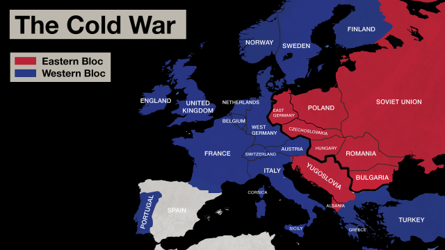
Trevor Dupuy’s article cited in my previous post, “Combat Data and the 3:1 Rule,” was the final salvo in a roaring, multi-year debate between two highly regarded members of the U.S. strategic and security studies academic communities, political scientist John Mearsheimer and military analyst/polymath Joshua Epstein. Carried out primarily in the pages of the academic journal International Security, Epstein and Mearsheimer argued the validity of the 3-1 rule and other analytical models with respect the NATO/Warsaw Pact military balance in Europe in the 1980s. Epstein cited Dupuy’s empirical research in support of his criticism of Mearsheimer’s reliance on the 3-1 rule. In turn, Mearsheimer questioned Dupuy’s data and conclusions to refute Epstein. Dupuy’s article defended his research and pointed out the errors in Mearsheimer’s assertions. With the publication of Dupuy’s rebuttal, the International Security editors called a time out on the debate thread.
These debates played a prominent role in the “renaissance of security studies” because they brought together scholars with different theoretical, methodological, and professional backgrounds to push forward a cohesive line of research that had clear implications for the conduct of contemporary defense policy. Just as importantly, the debate forced scholars to engage broader, fundamental issues. Is “military power” something that can be studied using static measures like force ratios, or does it require a more dynamic analysis? How should analysts evaluate the role of doctrine, or politics, or military strategy in determining the appropriate “balance”? What role should formal modeling play in formulating defense policy? What is the place for empirical analysis, and what are the strengths and limitations of existing data?[1]
It is well worth the time to revisit the contributions to the 1980s debate. I have included a bibliography below that is not exhaustive, but is a place to start. The collapse of the Soviet Union and the end of the Cold War diminished the intensity of the debates, which simmered through the 1990s and then were obscured during the counterterrorism/ counterinsurgency conflicts of the post-9/11 era. It is possible that the challenges posed by China and Russia amidst the ongoing “hybrid” conflict in Syria and Iraq may revive interest in interrogating the bases of military analyses in the U.S and the West. It is a discussion that is long overdue and potentially quite illuminating.
Canadian soldiers going “over the top” during an assault in the First World War. [History.com][This post was originally published on 1 December 2017.]
How many troops are needed to successfully attack or defend on the battlefield? There is a long-standing rule of thumb that holds that an attacker requires a 3-1 preponderance over a defender in combat in order to win. The aphorism is so widely accepted that few have questioned whether it is actually true or not.
Trevor Dupuy challenged the validity of the 3-1 rule on empirical grounds. He could find no historical substantiation to support it. In fact, his research on the question of force ratios suggested that there was a limit to the value of numerical preponderance on the battlefield.
TDI President Chris Lawrence has also challenged the 3-1 rule in his own work on the subject.
The validity of the 3-1 rule is no mere academic question. It underpins a great deal of U.S. military policy and warfighting doctrine. Yet, the only time the matter was seriously debated was in the 1980s with reference to the problem of defending Western Europe against the threat of Soviet military invasion.
It is probably long past due to seriously challenge the validity and usefulness of the 3-1 rule again.
The U.S. Army’s concept of combat power can be traced back to the thinking of British theorist J.F.C. Fuller, who collected his lectures and thoughts into the book, The Foundations of the Science of War (1926).
In a previous post, I critiqued the existing U.S. Army doctrinal method for calculating combat power. The ideas associated with the term “combat power” have been a part of U.S Army doctrine since the 1920s. However, the Army did not specifically define what combat power actually meant until the 1982 edition of FM 100-5 Operations, which introduced the AirLand Battle concept. So where did the Army’s notion of the concept originate? This post will trace the way it has been addressed in the capstone Field Manual (FM) 100-5 Operations series.
The first use of the phrase itself by the Army can be found in the 1939 edition of FM 100-5 Tentative Field Service Regulations, Operations, which replaced and updated the 1923 FSR. It appears just twice and was not explicitly defined in the text. As Boslego noted, however, even then the use of the term
highlighted a holistic view of combat power. This power was the sum of all factors which ultimately affected the ability of the soldiers to accomplish the mission. Interestingly, the authors of the 1939 edition did not focus solely on the physical objective of destroying the enemy. Instead, they sought to break the enemy’s power of resistance which connotes moral as well as physical factors.
This basic, implied definition of combat power as a combination of interconnected tangible physical and intangible moral factors could be found in all successive editions of FM 100-5 through 1968. The type and character of the factors comprising combat power evolved along with the Army’s experience of combat through this period, however. In addition to leadership, mobility, and firepower, the 1941 edition of FM 100-5 included “better armaments and equipment,” which reflected the Army’s initial impressions of the early “blitzkrieg” battles of World War II.
From World War II Through Korea
While FM 100-5 (1944) and FM 100-5 (1949) made no real changes with respect to describing combat power, the 1954 edition introduced significant new ideas in the wake of major combat operations in Korea, albeit still without actually defining the term. As with its predecessors, FM 100-5 (1954) posited combat power as a combination of firepower, maneuver, and leadership. For the first time, it defined the principles of mass, unity of command, maneuver, and surprise in terms of combat power. It linked the principle of the offensive, “only offensive action achieves decisive results,” with the enduring dictum that “offensive action requires the concentration of superior combat power at the decisive point and time.”
Boslego credited the authors of FM 100-5 (1954) with recognizing the non-linear nature of warfare and advising commanders to take a holistic perspective. He observed that they introduced the subtle but important understanding of combat power not as a fixed value, but as something relative and interactive between two forces in battle. Any calculation of combat power would be valid only in relation to the opposing combat force. “Relative combat power is dynamic and can be directly influenced by opposing commanders. It therefore must be analyzed by the commander in its potential relation to all other factors.” One of the fundamental ways a commander could shift the balance of combat power against an enemy was through maneuver: “Maneuver must be used to alter the relative combat power of military forces.”
The 1962 edition of FM 100-5 supplied a general definition of combat power that articulated the way the Army had been thinking about it since 1939.
Combat power is a combination of the physical means available to a commander and the moral strength of his command. It is significant only in relation to the combat power of the opposing forces. In applying the principles of war, the development and application of combat power are essential to decisive results.
It further refined the elements of combat power by redefining the principles of economy of force and security in terms of it as well.
dwelt heavily on the importance of dispersing forces to prevent major losses from a single nuclear strike, being highly mobile to mass at decisive points and being flexible in adjusting forces to the current situation. The terms dispersion, flexibility, and mobility were repeated so frequently in speeches, articles, and congressional testimony, that…they became a mantra. As a result, there was a lack of rigor in the Army concerning what they meant in general and how they would be applied on the tactical battlefield in particular.
The only change the 1968 edition made was to expand the elements of combat power to include “firepower, mobility, communications, condition of equipment, and status of supply,” which presaged an increasing focus on the technological aspects of combat and warfare.
The first major modification in the way the Army thought about combat power since before World War II was reflected in FM 100-5 (1976). These changes in turn prompted a significant reevaluation of the concept by then-U.S. Army Major Huba Wass de Czege. I will tackle how this resulted in the way combat power was redefined in the 1982 edition of FM 100-5 in a future post.
Consistent Scoring of Weapons and Aggregation of Forces: The Cornerstone of Dupuy’s Quantitative Analysis of Historical Land Battles by
James G. Taylor, PhD,
Dept. of Operations Research, Naval Postgraduate School
Introduction
Col. Trevor N. Dupuy was an American original, especially as regards the quantitative study of warfare. As with many prophets, he was not entirely appreciated in his own land, particularly its Military Operations Research (OR) community. However, after becoming rather familiar with the details of his mathematical modeling of ground combat based on historical data, I became aware of the basic scientific soundness of his approach. Unfortunately, his documentation of methodology was not always accepted by others, many of whom appeared to confuse lack of mathematical sophistication in his documentation with lack of scientific validity of his basic methodology.
The purpose of this brief paper is to review the salient points of Dupuy’s methodology from a system’s perspective, i.e., to view his methodology as a system, functioning as an organic whole to capture the essence of past combat experience (with an eye towards extrapolation into the future). The advantage of this perspective is that it immediately leads one to the conclusion that if one wants to use some functional relationship derived from Dupuy’s work, then one should use his methodologies for scoring weapons, aggregating forces, and adjusting for operational circumstances; since this consistency is the only guarantee of being able to reproduce historical results and to project them into the future.
Implications (of this system’s perspective on Dupuy’s work) for current DOD models will be discussed. In particular, the Military OR community has developed quantitative methods for imputing values to weapon systems based on their attrition capability against opposing forces and force interactions.[1] One such approach is the so-called antipotential-potential method[2] used in TACWAR[3] to score weapons. However, one should not expect such scores to provide valid casualty estimates when combined with historically derived functional relationships such as the so-called ATLAS casualty-rate curves[4] used in TACWAR, because a different “yard-stick” (i.e. measuring system for estimating the relative combat potential of opposing forces) was used to develop such a curve.
Overview of Dupuy’s Approach
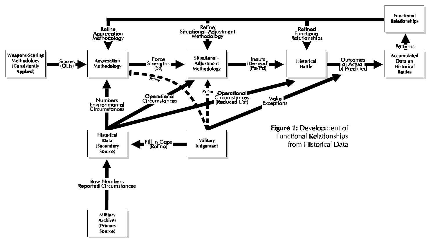
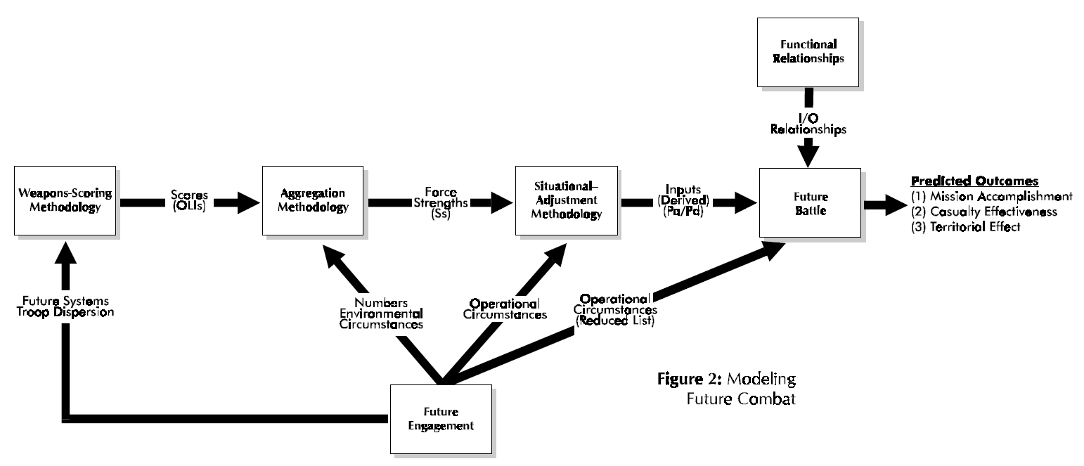
This section briefly outlines the salient features of Dupuy’s approach to the quantitative analysis and modeling of ground combat as embodied in his Tactical Numerical Deterministic Model (TNDM) and its predecessor the Quantified Judgment Model (QJM). The interested reader can find details in Dupuy [1979] (see also Dupuy [1985][5], [1987], [1990]). Here we will view Dupuy’s methodology from a system approach, which seeks to discern its various components and their interactions and to view these components as an organic whole. Essentially Dupuy’s approach involves the development of functional relationships from historical combat data (see Fig. 1) and then using these functional relationships to model future combat (see Fig, 2).
At the heart of Dupuy’s method is the investigation of historical battles and comparing the relationship of inputs (as quantified by relative combat power, denoted as Pa/Pd for that of the attacker relative to that of the defender in Fig. l)(e.g. see Dupuy [1979, pp. 59-64]) to outputs (as quantified by extent of mission accomplishment, casualty effectiveness, and territorial effectiveness; see Fig. 2) (e.g. see Dupuy [1979, pp. 47-50]), The salient point is that within this scheme, the main input[6] (i.e. relative combat power) to a historical battle is a derived quantity. It is computed from formulas that involve three essential aspects: (1) the scoring of weapons (e.g, see Dupuy [1979, Chapter 2 and also Appendix A]), (2) aggregation methodology for a force (e.g. see Dupuy [1979, pp. 43-46 and 202-203]), and (3) situational-adjustment methodology for determining the relative combat power of opposing forces (e.g. see Dupuy [1979, pp. 46-47 and 203-204]). In the force-aggregation step the effects on weapons of Dupuy’s environmental variables and one operational variable (air superiority) are considered[7], while in the situation-adjustment step the effects on forces of his behavioral variables[8] (aggregated into a single factor called the relative combat effectiveness value (CEV)) and also the other operational variables are considered (Dupuy [1987, pp. 86-89])
Figure 1.
Moreover, any functional relationships developed by Dupuy depend (unless shown otherwise) on his computational system for derived quantities, namely OLls, force strengths, and relative combat power. Thus, Dupuy’s results depend in an essential manner on his overall computational system described immediately above. Consequently, any such functional relationship (e.g. casualty-rate curve) directly or indirectly derivative from Dupuy‘s work should still use his computational methodology for determination of independent-variable values.
Fig l also reveals another important aspect of Dupuy’s work, the development of reliable data on historical battles, Military judgment plays an essential role in this development of such historical data for a variety of reasons. Dupuy was essentially the only source of new secondary historical data developed from primary sources (see McQuie [1970] for further details). These primary sources are well known to be both incomplete and inconsistent, so that military judgment must be used to fill in the many gaps and reconcile observed inconsistencies. Moreover, military judgment also generates the working hypotheses for model development (e.g. identification of significant variables).
At the heart of Dupuy’s quantitative investigation of historical battles and subsequent model development is his own weapons-scoring methodology, which slowly evolved out of study efforts by the Historical Evaluation Research Organization (HERO) and its successor organizations (cf. HERO [1967] and compare with Dupuy [1979]). Early HERO [1967, pp. 7-8] work revealed that what one would today call weapons scores developed by other organizations were so poorly documented that HERO had to create its own methodology for developing the relative lethality of weapons, which eventually evolved into Dupuy’s Operational Lethality Indices (OLIs). Dupuy realized that his method was arbitrary (as indeed is its counterpart, called the operational definition, in formal scientific work), but felt that this would be ameliorated if the weapons-scoring methodology be consistently applied to historical battles. Unfortunately, this point is not clearly stated in Dupuy’s formal writings, although it was clearly (and compellingly) made by him in numerous briefings that this author heard over the years.
Figure 2.
In other words, from a system’s perspective, the functional relationships developed by Colonel Dupuy are part of his analysis system that includes this weapons-scoring methodology consistently applied (see Fig. l again). The derived functional relationships do not stand alone (unless further empirical analysis shows them to hold for any weapons-scoring methodology), but function in concert with computational procedures. Another essential part of this system is Dupuy‘s aggregation methodology, which combines numbers, environmental circumstances, and weapons scores to compute the strength (S) of a military force. A key innovation by Colonel Dupuy [1979, pp. 202- 203] was to use a nonlinear (more precisely, a piecewise-linear) model for certain elements of force strength. This innovation precluded the occurrence of military absurdities such as air firepower being fully substitutable for ground firepower, antitank weapons being fully effective when armor targets are lacking, etc‘ The final part of this computational system is Dupuy’s situational-adjustment methodology, which combines the effects of operational circumstances with force strengths to determine relative combat power, e.g. Pa/Pd.
To recapitulate, the determination of an Operational Lethality Index (OLI) for a weapon involves the combination of weapon lethality, quantified in terms of a Theoretical Lethality Index (TLI) (e.g. see Dupuy [1987, p. 84]), and troop dispersion[9] (e.g. see Dupuy [1987, pp. 84- 85]). Weapons scores (i.e. the OLIs) are then combined with numbers (own side and enemy) and combat- environment factors to yield force strength. Six[10] different categories of weapons are aggregated, with nonlinear (i.e. piecewise-linear) models being used for the following three categories of weapons: antitank, air defense, and air firepower (i.e. c1ose—air support). Operational, e.g. mobility, posture, surprise, etc. (Dupuy [1987, p. 87]), and behavioral variables (quantified as a relative combat effectiveness value (CEV)) are then applied to force strength to determine a side’s combat-power potential.
Requirement for Consistent Scoring of Weapons, Force Aggregation, and Situational Adjustment for Operational Circumstances
The salient point to be gleaned from Fig.1 and 2 is that the same (or at least consistent) weapons—scoring, aggregation, and situational—adjustment methodologies be used for both developing functional relationships and then playing them to model future combat. The corresponding computational methods function as a system (organic whole) for determining relative combat power, e.g. Pa/Pd. For the development of functional relationships from historical data, a force ratio (relative combat power of the two opposing sides, e.g. attacker’s combat power divided by that of the defender, Pa/Pd is computed (i.e. it is a derived quantity) as the independent variable, with observed combat outcome being the dependent variable. Thus, as discussed above, this force ratio depends on the methodologies for scoring weapons, aggregating force strengths, and adjusting a force’s combat power for the operational circumstances of the engagement. It is a priori not clear that different scoring, aggregation, and situational-adjustment methodologies will lead to similar derived values. If such different computational procedures were to be used, these derived values should be recomputed and the corresponding functional relationships rederived and replotted.
However, users of the Tactical Numerical Deterministic Model (TNDM) (or for that matter, its predecessor, the Quantified Judgment Model (QJM)) need not worry about this point because it was apparently meticulously observed by Colonel Dupuy in all his work. However, portions of his work have found their way into a surprisingly large number of DOD models (usually not explicitly acknowledged), but the context and range of validity of historical results have been largely ignored by others. The need for recalibration of the historical data and corresponding functional relationships has not been considered in applying Dupuy’s results for some important current DOD models.
Implications for Current DOD Models
A number of important current DOD models (namely, TACWAR and JICM discussed below) make use of some of Dupuy’s historical results without recalibrating functional relationships such as loss rates and rates of advance as a function of some force ratio (e.g. Pa/Pd). As discussed above, it is not clear that such a procedure will capture the essence of past combat experience. Moreover, in calculating losses, Dupuy first determines personnel losses (expressed as a percent loss of personnel strength, i.e., number of combatants on a side) and then calculates equipment losses as a function of this casualty rate (e.g., see Dupuy [1971, pp. 219-223], also [1990, Chapters 5 through 7][11]). These latter functional relationships are apparently not observed in the models discussed below. In fact, only Dupuy (going back to Dupuy [1979][12] takes personnel losses to depend on a force ratio and other pertinent variables, with materiel losses being taken as derivative from this casualty rate.
For example, TACWAR determines personnel losses[13] by computing a force ratio and then consulting an appropriate casualty-rate curve (referred to as empirical data), much in the same fashion as ATLAS did[14]. However, such a force ratio is computed using a linear model with weapon values determined by the so-called antipotential-potential method[15]. Unfortunately, this procedure may not be consistent with how the empirical data (i.e. the casualty-rate curves) was developed. Further research is required to demonstrate that valid casualty estimates are obtained when different weapon scoring, aggregation, and situational-adjustment methodologies are used to develop casualty-rate curves from historical data and to use them to assess losses in aggregated combat models. Furthermore, TACWAR does not use Dupuy’s model for equipment losses (see above), although it does purport, as just noted above, to use “historical data” (e.g., see Kerlin et al. [1975, p. 22]) to compute personnel losses as a function (among other things) of a force ratio (given by a linear relationship), involving close air support values in a way never used by Dupuy. Although their force-ratio determination methodology does have logical and mathematical merit, it is not the way that the historical data was developed.
Moreover, RAND (Allen [1992]) has more recently developed what is called the situational force scoring (SFS) methodology for calculating force ratios in large-scale, aggregated-force combat situations to determine loss and movement rates. Here, SFS refers essentially to a force- aggregation and situation-adjustment methodology, which has many conceptual elements in common with Dupuy‘s methodology (except, most notably, extensive testing against historical data, especially documentation of such efforts). This SFS was originally developed for RSAS[16] and is today used in JICM[17]. It also apparently uses a weapon-scoring system developed at RAND[18]. It purports (no documentation given [citation of unpublished work]) to be consistent with historical data (including the ATLAS casualty-rate curves) (Allen [1992, p.41]), but again no consideration is given to recalibration of historical results for different weapon scoring, force-aggregation, and situational-adjustment methodologies. SFS emphasizes adjusting force strengths according to operational circumstances (the “situation”) of the engagement (including surprise), with many innovative ideas (but in some major ways has little connection with previous work of others[19]). The resulting model contains many more details than historical combat data would support. It also is methodology that differs in many essential ways from that used previously by any investigator. In particular, it is doubtful that it develops force ratios in a manner consistent with Dupuy’s work.
Final Comments
Use of (sophisticated) mathematics for modeling past historical combat (and extrapolating it into the future for planning purposes) is no reason for ignoring Dupuy’s work. One would think that the current Military OR community would try to understand Dupuy’s work before trying to improve and extend it. In particular, Colonel Dupuy’s various computational procedures (including constants) must be considered as an organic whole (i.e. a system) supporting the development of functional relationships. If one ignores this computational system and simply tries to use some isolated aspect, the result may be interesting and even logically sound, but it probably lacks any scientific validity.
REFERENCES
P. Allen, “Situational Force Scoring: Accounting for Combined Arms Effects in Aggregate Combat Models,” N-3423-NA, The RAND Corporation, Santa Monica, CA, 1992.
L. B. Anderson, “A Briefing on Anti-Potential Potential (The Eigen-value Method for Computing Weapon Values), WP-2, Project 23-31, Institute for Defense Analyses, Arlington, VA, March 1974.
B. W. Bennett, et al, “RSAS 4.6 Summary,” N-3534-NA, The RAND Corporation, Santa Monica, CA, 1992.
B. W. Bennett, A. M. Bullock, D. B. Fox, C. M. Jones, J. Schrader, R. Weissler, and B. A. Wilson, “JICM 1.0 Summary,” MR-383-NA, The RAND Corporation, Santa Monica, CA, 1994.
P. K. Davis and J. A. Winnefeld, “The RAND Strategic Assessment Center: An Overview and Interim Conclusions About Utility and Development Options,” R-2945-DNA, The RAND Corporation, Santa Monica, CA, March 1983.
T.N, Dupuy, Numbers. Predictions and War: Using History to Evaluate Combat Factors and Predict the Outcome of Battles, The Bobbs-Merrill Company, Indianapolis/New York, 1979,
T.N. Dupuy, Numbers Predictions and War, Revised Edition, HERO Books, Fairfax, VA 1985.
T.N. Dupuy, Understanding War: History and Theory of Combat, Paragon House Publishers, New York, 1987.
T.N. Dupuy, Attrition: Forecasting Battle Casualties and Equipment Losses in Modem War, HERO Books, Fairfax, VA, 1990.
General Research Corporation (GRC), “A Hierarchy of Combat Analysis Models,” McLean, VA, January 1973.
Historical Evaluation and Research Organization (HERO), “Average Casualty Rates for War Games, Based on Historical Data,” 3 Volumes in 1, Dunn Loring, VA, February 1967.
E. P. Kerlin and R. H. Cole, “ATLAS: A Tactical, Logistical, and Air Simulation: Documentation and User’s Guide,” RAC-TP-338, Research Analysis Corporation, McLean, VA, April 1969 (AD 850 355).
E.P. Kerlin, L.A. Schmidt, A.J. Rolfe, M.J. Hutzler, and D,L. Moody, “The IDA Tactical Warfare Model: A Theater-Level Model of Conventional, Nuclear, and Chemical Warfare, Volume II- Detailed Description” R-21 1, Institute for Defense Analyses, Arlington, VA, October 1975 (AD B009 692L).
R. McQuie, “Military History and Mathematical Analysis,” Military Review 50, No, 5, 8-17 (1970).
S.M. Robinson, “Shadow Prices for Measures of Effectiveness, I: Linear Model,” Operations Research 41, 518-535 (1993).
J.G. Taylor, Lanchester Models of Warfare. Vols, I & II. Operations Research Society of America, Alexandria, VA, 1983. (a)
J.G. Taylor, “A Lanchester-Type Aggregated-Force Model of Conventional Ground Combat,” Naval Research Logistics Quarterly 30, 237-260 (1983). (b)
NOTES
[1] For example, see Taylor [1983a, Section 7.18], which contains a number of examples. The basic references given there may be more accessible through Robinson [I993].
[2] This term was apparently coined by L.B. Anderson [I974] (see also Kerlin et al. [1975, Chapter I, Section D.3]).
[3] The Tactical Warfare (TACWAR) model is a theater-level, joint-warfare, computer-based combat model that is currently used for decision support by the Joint Staff and essentially all CINC staffs. It was originally developed by the Institute for Defense Analyses in the mid-1970s (see Kerlin et al. [1975]), originally referred to as TACNUC, which has been continually upgraded until (and including) the present day.
[4] For example, see Kerlin and Cole [1969], GRC [1973, Fig. 6-6], or Taylor [1983b, Fig. 5] (also Taylor [1983a, Section 7.13]).
[5] The only apparent difference between Dupuy [1979] and Dupuy [1985] is the addition of an appendix (Appendix C “Modified Quantified Judgment Analysis of the Bekaa Valley Battle”) to the end of the latter (pp. 241-251). Hence, the page content is apparently the same for these two books for pp. 1-239.
[6] Technically speaking, one also has the engagement type and possibly several other descriptors (denoted in Fig. 1 as reduced list of operational circumstances) as other inputs to a historical battle.
[7] In Dupuy [1979, e.g. pp. 43-46] only environmental variables are mentioned, although basically the same formulas underlie both Dupuy [1979] and Dupuy [1987]. For simplicity, Fig. 1 and 2 follow this usage and employ the term “environmental circumstances.”
[8] In Dupuy [1979, e.g. pp. 46-47] only operational variables are mentioned, although basically the same formulas underlie both Dupuy [1979] and Dupuy [1987]. For simplicity, Fig. 1 and 2 follow this usage and employ the term “operational circumstances.”
[9] Chris Lawrence has kindly brought to my attention that since the same value for troop dispersion from an historical period (e.g. see Dupuy [1987, p. 84]) is used for both the attacker and also the defender, troop dispersion does not actually affect the determination of relative combat power PM/Pd.
[10] Eight different weapon types are considered, with three being classified as infantry weapons (e.g. see Dupuy [1979, pp, 43-44], [1981 pp. 85-86]).
[11] Chris Lawrence has kindly informed me that Dupuy‘s work on relating equipment losses to personnel losses goes back to the early 1970s and even earlier (e.g. see HERO [1966]). Moreover, Dupuy‘s [1992] book Future Wars gives some additional empirical evidence concerning the dependence of equipment losses on casualty rates.
[12] But actually going back much earlier as pointed out in the previous footnote.
[13] See Kerlin et al. [1975, Chapter I, Section D.l].
[14] See Footnote 4 above.
[15] See Kerlin et al. [1975, Chapter I, Section D.3]; see also Footnotes 1 and 2 above.
[16] The RAND Strategy Assessment System (RSAS) is a multi-theater aggregated combat model developed at RAND in the early l980s (for further details see Davis and Winnefeld [1983] and Bennett et al. [1992]). It evolved into the Joint Integrated Contingency Model (JICM), which is a post-Cold War redesign of the RSAS (starting in FY92).
[17] The Joint Integrated Contingency Model (JICM) is a game-structured computer-based combat model of major regional contingencies and higher-level conflicts, covering strategic mobility, regional conventional and nuclear warfare in multiple theaters, naval warfare, and strategic nuclear warfare (for further details, see Bennett et al. [1994]).
[18] RAND apparently replaced one weapon-scoring system by another (e.g. see Allen [1992, pp. 9, l5, and 87-89]) without making any other changes in their SFS System.
[19] For example, both Dupuy’s early HERO work (e.g. see Dupuy [1967]), reworks of these results by the Research Analysis Corporation (RAC) (e.g. see RAC [1973, Fig. 6-6]), and Dupuy’s later work (e.g. see Dupuy [1979]) considered daily fractional casualties for the attacker and also for the defender as basic casualty-outcome descriptors (see also Taylor [1983b]). However, RAND does not do this, but considers the defender’s loss rate and a casualty exchange ratio as being the basic casualty-production descriptors (Allen [1992, pp. 41-42]). The great value of using the former set of descriptors (i.e. attacker and defender fractional loss rates) is that not only is casualty assessment more straight forward (especially development of functional relationships from historical data) but also qualitative model behavior is readily deduced (see Taylor [1983b] for further details).
Allied force dispositions at the Battle of Anzio, on 1 February 1944. [U.S. Army/Wikipedia]
[The article below is reprinted from History, Numbers And War: A HERO Journal, Vol. 1, No. 1, Spring 1977, pp. 34-52]
The Lanchester Equations and Historical Warfare: An Analysis of Sixty World War II Land Engagements
By Janice B. Fain
Background and Objectives
The method by which combat losses are computed is one of the most critical parts of any combat model. The Lanchester equations, which state that a unit’s combat losses depend on the size of its opponent, are widely used for this purpose.
In addition to their use in complex dynamic simulations of warfare, the Lanchester equations have also sewed as simple mathematical models. In fact, during the last decade or so there has been an explosion of theoretical developments based on them. By now their variations and modifications are numerous, and “Lanchester theory” has become almost a separate branch of applied mathematics. However, compared with the effort devoted to theoretical developments, there has been relatively little empirical testing of the basic thesis that combat losses are related to force sizes.
One of the first empirical studies of the Lanchester equations was Engel’s classic work on the Iwo Jima campaign in which he found a reasonable fit between computed and actual U.S. casualties (Note 1). Later studies were somewhat less supportive (Notes 2 and 3), but an investigation of Korean war battles showed that, when the simulated combat units were constrained to follow the tactics of their historical counterparts, casualties during combat could be predicted to within 1 to 13 percent (Note 4).
Taken together, these various studies suggest that, while the Lanchester equations may be poor descriptors of large battles extending over periods during which the forces were not constantly in combat, they may be adequate for predicting losses while the forces are actually engaged in fighting. The purpose of the work reported here is to investigate 60 carefully selected World War II engagements. Since the durations of these battles were short (typically two to three days), it was expected that the Lanchester equations would show a closer fit than was found in studies of larger battles. In particular, one of the objectives was to repeat, in part, Willard’s work on battles of the historical past (Note 3).
The Data Base
Probably the most nearly complete and accurate collection of combat data is the data on World War II compiled by the Historical Evaluation and Research Organization (HERO). From their data HERO analysts selected, for quantitative analysis, the following 60 engagements from four major Italian campaigns:
Salerno, 9-18 Sep 1943, 9 engagements
Volturno, 12 Oct-8 Dec 1943, 20 engagements
Anzio, 22 Jan-29 Feb 1944, 11 engagements
Rome, 14 May-4 June 1944, 20 engagements
The complete data base is described in a HERO report (Note 5). The work described here is not the first analysis of these data. Statistical analyses of weapon effectiveness and the testing of a combat model (the Quantified Judgment Method, QJM) have been carried out (Note 6). The work discussed here examines these engagements from the viewpoint of the Lanchester equations to consider the question: “Are casualties during combat related to the numbers of men in the opposing forces?”
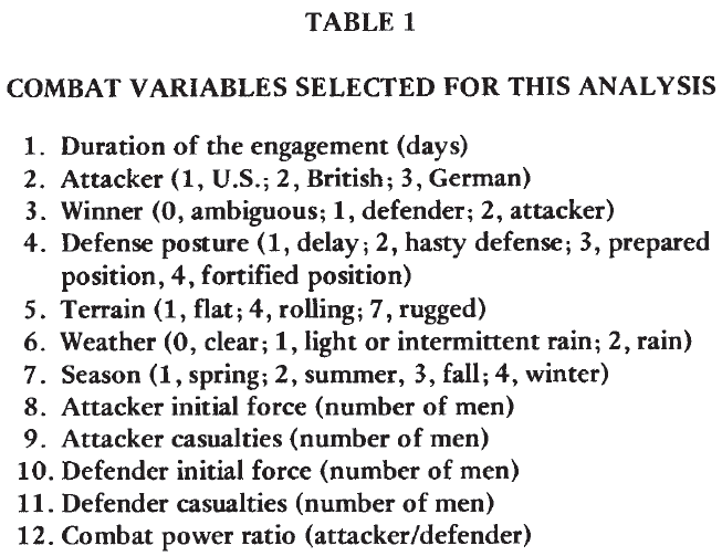
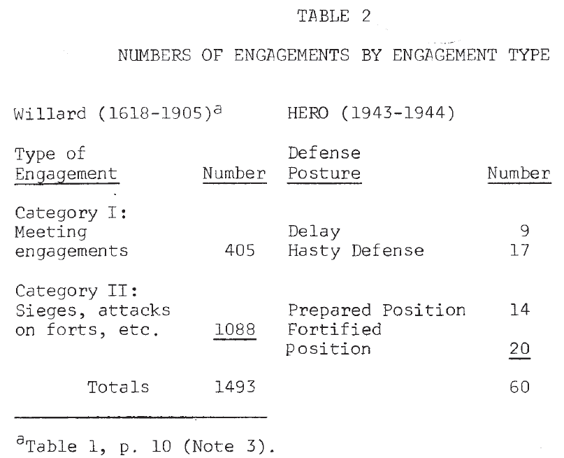
The variables chosen for this analysis are shown in Table 1. The “winners” of the engagements were specified by HERO on the basis of casualties suffered, distance advanced, and subjective estimates of the percentage of the commander’s objective achieved. Variable 12, the Combat Power Ratio, is based on the Operational Lethality Indices (OLI) of the units (Note 7).
The general characteristics of the engagements are briefly described. Of the 60, there were 19 attacks by British forces, 28 by U.S. forces, and 13 by German forces. The attacker was successful in 34 cases; the defender, in 23; and the outcomes of 3 were ambiguous. With respect to terrain, 19 engagements occurred in flat terrain; 24 in rolling, or intermediate, terrain; and 17 in rugged, or difficult, terrain. Clear weather prevailed in 40 cases; 13 engagements were fought in light or intermittent rain; and 7 in medium or heavy rain. There were 28 spring and summer engagements and 32 fall and winter engagements.
Comparison of World War II Engagements With Historical Battles
Since one purpose of this work is to repeat, in part, Willard’s analysis, comparison of these World War II engagements with the historical battles (1618-1905) studied by him will be useful. Table 2 shows a comparison of the distribution of battles by type. Willard’s cases were divided into two categories: I. meeting engagements, and II. sieges, attacks on forts, and similar operations. HERO’s World War II engagements were divided into four types based on the posture of the defender: 1. delay, 2. hasty defense, 3. prepared position, and 4. fortified position. If postures 1 and 2 are considered very roughly equivalent to Willard’s category I, then in both data sets the division into the two gross categories is approximately even.
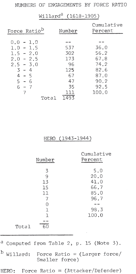
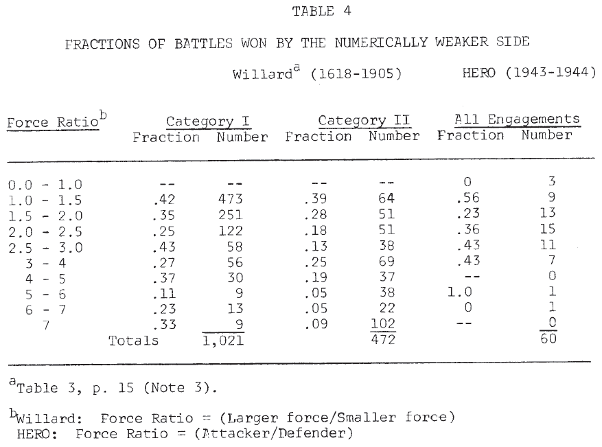
The distribution of engagements across force ratios, given in Table 3, indicated some differences. Willard’s engagements tend to cluster at the lower end of the scale (1-2) and at the higher end (4 and above), while the majority of the World War II engagements were found in mid-range (1.5 – 4) (Note 8). The frequency with which the numerically inferior force achieved victory is shown in Table 4. It is seen that in neither data set are force ratios good predictors of success in battle (Note 9).
Table 3.
Results of the Analysis Willard’s Correlation Analysis
There are two forms of the Lanchester equations. One represents the case in which firing units on both sides know the locations of their opponents and can shift their fire to a new target when a “kill” is achieved. This leads to the “square” law where the loss rate is proportional to the opponent’s size. The second form represents that situation in which only the general location of the opponent is known. This leads to the “linear” law in which the loss rate is proportional to the product of both force sizes.
As Willard points out, large battles are made up of many smaller fights. Some of these obey one law while others obey the other, so that the overall result should be a combination of the two. Starting with a general formulation of Lanchester’s equations, where g is the exponent of the target unit’s size (that is, g is 0 for the square law and 1 for the linear law), he derives the following linear equation:
log (nc/mc) = log E + g log (mo/no) (1)
where nc and mc are the casualties, E is related to the exchange ratio, and mo and no are the initial force sizes. Linear regression produces a value for g. However, instead of lying between 0 and 1, as expected, the) g‘s range from -.27 to -.87, with the majority lying around -.5. (Willard obtains several values for g by dividing his data base in various ways—by force ratio, by casualty ratio, by historical period, and so forth.) A negative g value is unpleasant. As Willard notes:
Military theorists should be disconcerted to find g < 0, for in this range the results seem to imply that if the Lanchester formulation is valid, the casualty-producing power of troops increases as they suffer casualties (Note 3).
From his results, Willard concludes that his analysis does not justify the use of Lanchester equations in large-scale situations (Note 10).
Analysis of the World War II Engagements
Willard’s computations were repeated for the HERO data set. For these engagements, regression produced a value of -.594 for g (Note 11), in striking agreement with Willard’s results. Following his reasoning would lead to the conclusion that either the Lanchester equations do not represent these engagements, or that the casualty producing power of forces increases as their size decreases.
However, since the Lanchester equations are so convenient analytically and their use is so widespread, it appeared worthwhile to reconsider this conclusion. In deriving equation (1), Willard used binomial expansions in which he retained only the leading terms. It seemed possible that the poor results might he due, in part, to this approximation. If the first two terms of these expansions are retained, the following equation results:
log (nc/mc) = log E + log (Mo-mc)/(no-nc) (2)
Repeating this regression on the basis of this equation leads to g = -.413 (Note 12), hardly an improvement over the initial results.
A second attempt was made to salvage this approach. Starting with raw OLI scores (Note 7), HERO analysts have computed “combat potentials” for both sides in these engagements, taking into account the operational factors of posture, vulnerability, and mobility; environmental factors like weather, season, and terrain; and (when the record warrants) psychological factors like troop training, morale, and the quality of leadership. Replacing the factor (mo/no) in Equation (1) by the combat power ratio produces the result) g = .466 (Note 13).
While this is an apparent improvement in the value of g, it is achieved at the expense of somewhat distorting the Lanchester concept. It does preserve the functional form of the equations, but it requires a somewhat strange definition of “killing rates.”
Analysis Based on the Differential Lanchester Equations
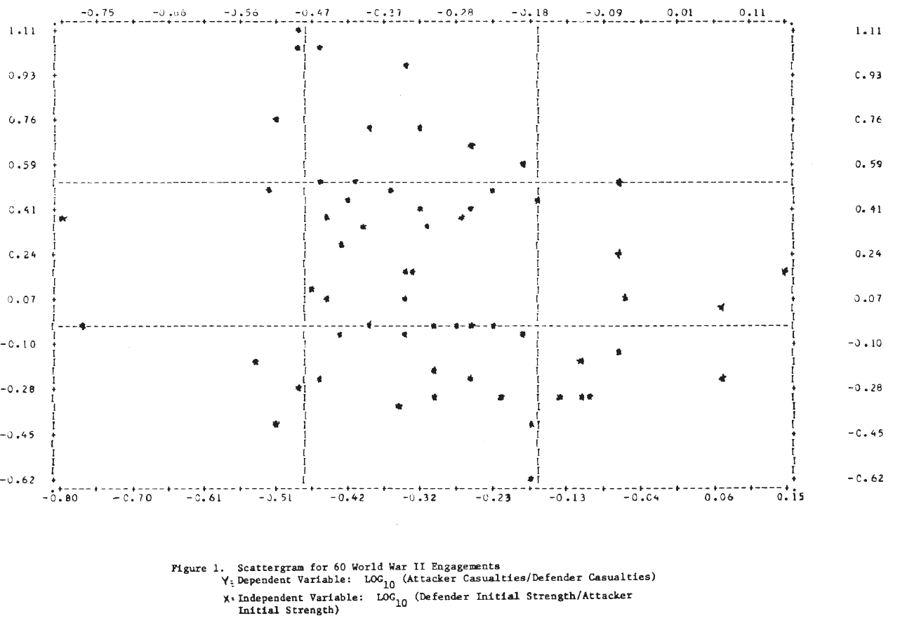
Analysis of the type carried out by Willard appears to produce very poor results for these World War II engagements. Part of the reason for this is apparent from Figure 1, which shows the scatterplot of the dependent variable, log (nc/mc), against the independent variable, log (mo/no). It is clear that no straight line will fit these data very well, and one with a positive slope would not be much worse than the “best” line found by regression. To expect the exponent to account for the wide variation in these data seems unreasonable.
Here, a simpler approach will be taken. Rather than use the data to attempt to discriminate directly between the square and the linear laws, they will be used to estimate linear coefficients under each assumption in turn, starting with the differential formulation rather than the integrated equations used by Willard.
In their simplest differential form, the Lanchester equations may be written;
Square Law; dA/dt = -kdD and dD/dt = kaA (3)
Linear law: dA/dt = -k’dAD and dD/dt = k’aAD (4)
where
A(D) is the size of the attacker (defender)
dA/dt (dD/dt) is the attacker’s (defender’s) loss rate,
ka, k’a (kd, k’d) are the attacker’s (defender’s) killing rates
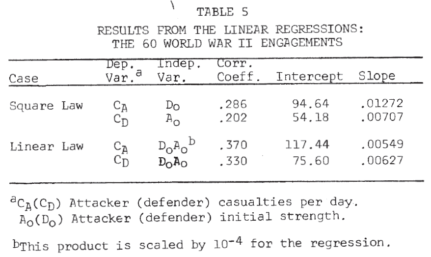
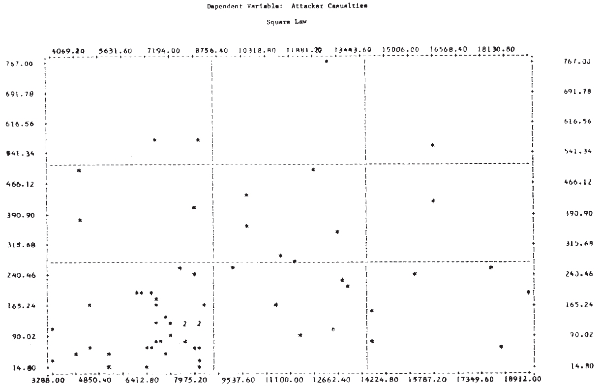
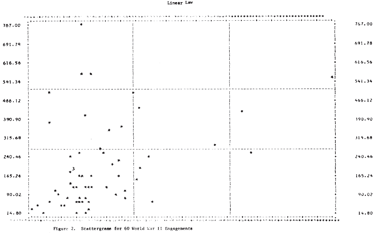
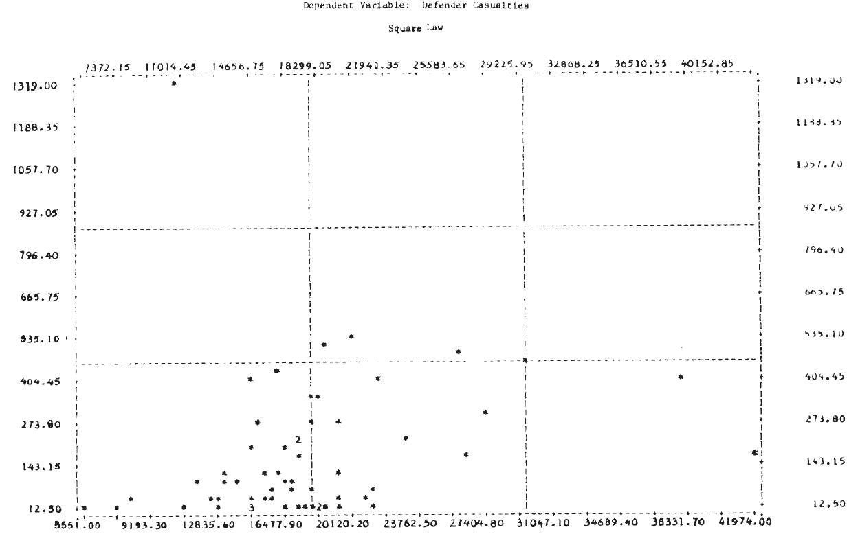
For this analysis, the day is taken as the basic time unit, and the loss rate per day is approximated by the casualties per day. Results of the linear regressions are given in Table 5. No conclusions should be drawn from the fact that the correlation coefficients are higher in the linear law case since this is expected for purely technical reasons (Note 14). A better picture of the relationships is again provided by the scatterplots in Figure 2. It is clear from these plots that, as in the case of the logarithmic forms, a single straight line will not fit the entire set of 60 engagements for either of the dependent variables.
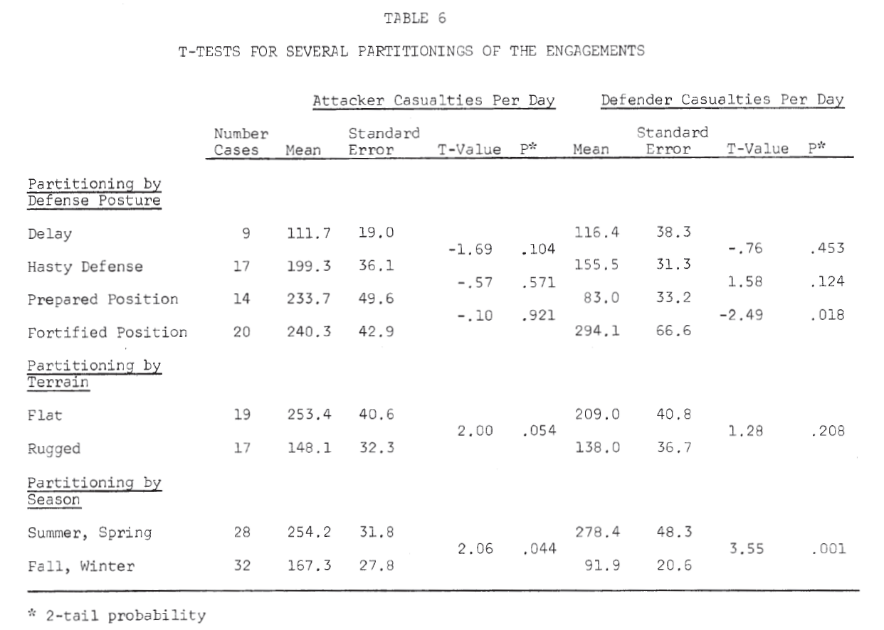
To investigate ways in which the data set might profitably be subdivided for analysis, T-tests of the means of the dependent variable were made for several partitionings of the data set. The results, shown in Table 6, suggest that dividing the engagements by defense posture might prove worthwhile.
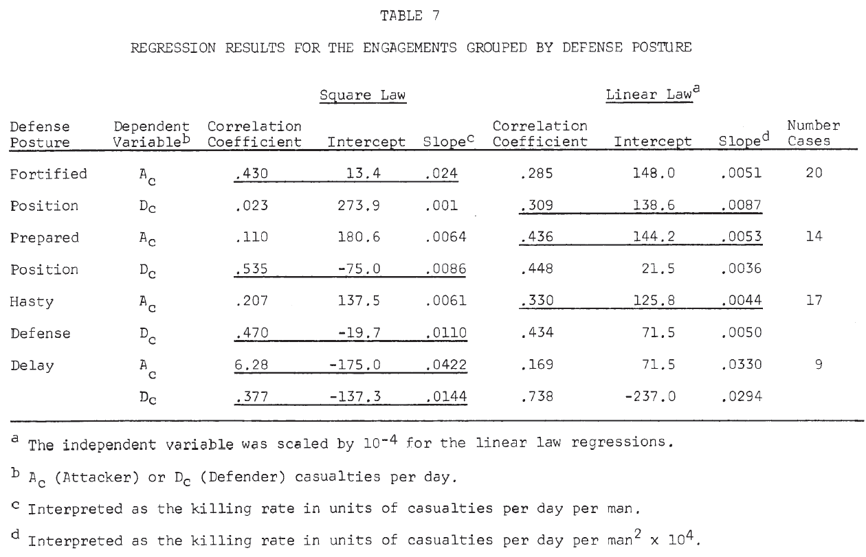
Results of the linear regressions by defense posture are shown in Table 7. For each posture, the equation that seemed to give a better fit to the data is underlined (Note 15). From this table, the following very tentative conclusions might be drawn:
In an attack on a fortified position, the attacker suffers casualties by the square law; the defender suffers casualties by the linear law. That is, the defender is aware of the attacker’s position, while the attacker knows only the general location of the defender. (This is similar to Deitchman’s guerrilla model. Note 16).
This situation is apparently reversed in the cases of attacks on prepared positions and hasty defenses.
Delaying situations seem to be treated better by the square law for both attacker and defender.
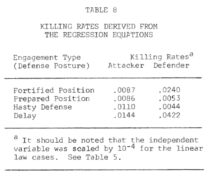
Table 8 summarizes the killing rates by defense posture. The defender has a much higher killing rate than the attacker (almost 3 to 1) in a fortified position. In a prepared position and hasty defense, the attacker appears to have the advantage. However, in a delaying action, the defender’s killing rate is again greater than the attacker’s (Note 17).
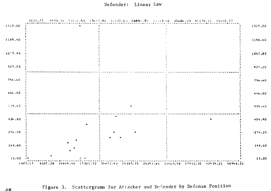
Figure 3 shows the scatterplots for these cases. Examination of these plots suggests that a tentative answer to the study question posed above might be: “Yes, casualties do appear to be related to the force sizes, but the relationship may not be a simple linear one.”
In several of these plots it appears that two or more functional forms may be involved. Consider, for example, the defender‘s casualties as a function of the attacker’s initial strength in the case of a hasty defense. This plot is repeated in Figure 4, where the points appear to fit the curves sketched there. It would appear that there are at least two, possibly three, separate relationships. Also on that plot, the individual engagements have been identified, and it is interesting to note that on the curve marked (1), five of the seven attacks were made by Germans—four of them from the Salerno campaign. It would appear from this that German attacks are associated with higher than average defender casualties for the attacking force size. Since there are so few data points, this cannot be more than a hint or interesting suggestion.
Future Research
This work suggests two conclusions that might have an impact on future lines of research on combat dynamics:
Tactics appear to be an important determinant of combat results. This conclusion, in itself, does not appear startling, at least not to the military. However, it does not always seem to have been the case that tactical questions have been considered seriously by analysts in their studies of the effects of varying force levels and force mixes.
Historical data of this type offer rich opportunities for studying the effects of tactics. For example, consideration of the narrative accounts of these battles might permit re-coding the engagements into a larger, more sensitive set of engagement categories. (It would, of course, then be highly desirable to add more engagements to the data set.)
While predictions of the future are always dangerous, I would nevertheless like to suggest what appears to be a possible trend. While military analysis of the past two decades has focused almost exclusively on the hardware of weapons systems, at least part of our future analysis will be devoted to the more behavioral aspects of combat.
Janice Bloom Fain, a Senior Associate of CACI, lnc., is a physicist whose special interests are in the applications of computer simulation techniques to industrial and military operations; she is the author of numerous reports and articles in this field. This paper was presented by Dr. Fain at the Military Operations Research Symposium at Fort Eustis, Virginia.
[5.] HERO, “A Study of the Relationship of Tactical Air Support Operations to Land Combat, Appendix B, Historical Data Base.” Historical Evaluation and Research Organization, report prepared for the Defense Operational Analysis Establishment, U.K.T.S.D., Contract D-4052 (1971).
[6.] T. N. Dupuy, The Quantified Judgment Method of Analysis of Historical Combat Data, HERO Monograph, (January 1973); HERO, “Statistical Inference in Analysis in Combat,” Annex F, Historical Data Research on Tactical Air Operations, prepared for Headquarters USAF, Assistant Chief of Staff for Studies and Analysis, Contract No. F-44620-70-C-0058 (1972).
[7.] The Operational Lethality Index (OLI) is a measure of weapon effectiveness developed by HERO.
[8.] Since Willard’s data did not indicate which side was the attacker, his force ratio is defined to be (larger force/smaller force). The HERO force ratio is (attacker/defender).
[9.] Since the criteria for success may have been rather different for the two sets of battles, this comparison may not be very meaningful.
[10.] This work includes more complex analysis in which the possibility that the two forces may be engaging in different types of combat is considered, leading to the use of two exponents rather than the single one, Stochastic combat processes are also treated.
[11.] Correlation coefficient = -.262;
Intercept = .00115; slope = -.594.
[12.] Correlation coefficient = -.184;
Intercept = .0539; slope = -,413.
[13.] Correlation coefficient = .303;
Intercept = -.638; slope = .466.
[14.] Correlation coefficients for the linear law are inflated with respect to the square law since the independent variable is a product of force sizes and, thus, has a higher variance than the single force size unit in the square law case.
[15.] This is a subjective judgment based on the following considerations Since the correlation coefficient is inflated for the linear law, when it is lower the square law case is chosen. When the linear law correlation coefficient is higher, the case with the intercept closer to 0 is chosen.
[17.] As pointed out by Mr. Alan Washburn, who prepared a critique on this paper, when comparing numerical values of the square law and linear law killing rates, the differences in units must be considered. (See footnotes to Table 7).
French retreat from Russia in 1812 by Illarion Mikhailovich Pryanishnikov (1812) [Wikipedia]
After discussing with Chris the series of recent posts on the subject of breakpoints, it seemed appropriate to provide a better definition of exactly what a breakpoint is.
Dorothy Kneeland Clark was the first to define the notion of a breakpoint in her study, Casualties as a Measure of the Loss of Combat Effectiveness of an Infantry Battalion (Operations Research Office, The Johns Hopkins University: Baltimore, 1954). She found it was not quite as clear-cut as it seemed and the working definition she arrived at was based on discussions and the specific combat outcomes she found in her data set [pp 9-12].
DETERMINATION OF BREAKPOINT
The following definitions were developed out of many discussions. A unit is considered to have lost its combat effectiveness when it is unable to carry out its mission. The onset of this inability constitutes a breakpoint. A unit’s mission is the objective assigned in the current operations order or any other instructional directive, written or verbal. The objective may be, for example, to attack in order to take certain positions, or to defend certain positions.
How does one determine when a unit is unable to carry out its mission? The obvious indication is a change in operational directive: the unit is ordered to stop short of its original goal, to hold instead of attack, to withdraw instead of hold. But one or more extraneous elements may cause the issue of such orders:
(1) Some other unit taking part in the operation may have lost its combat effectiveness, and its predicament may force changes, in the tactical plan. For example the inability of one infantry battalion to take a hill may require that the two adjoining battalions be stopped to prevent exposing their flanks by advancing beyond it.
(2) A unit may have been assigned an objective on the basis of a G-2 estimate of enemy weakness which, as the action proceeds, proves to have been over-optimistic. The operations plan may, therefore, be revised before the unit has carried out its orders to the point of losing combat effectiveness.
(3) The commanding officer, for reasons quite apart from the tactical attrition, may change his operations plan. For instance, General Ridgway in May 1951 was obliged to cancel his plans for a major offensive north of the 38th parallel in Korea in obedience to top level orders dictated by political considerations.
(4) Even if the supposed combat effectiveness of the unit is the determining factor in the issuance of a revised operations order, a serious difficulty in evaluating the situation remains. The commanding officer’s decision is necessarily made on the basis of information available to him plus his estimate of his unit’s capacities. Either or both of these bases may be faulty. The order may belatedly recognize a collapse which has in factor occurred hours earlier, or a commanding officer may withdraw a unit which could hold for a much longer time.
It was usually not hard to discover when changes in orders resulted from conditions such as the first three listed above, but it proved extremely difficult to distinguish between revised orders based on a correct appraisal of the unit’s combat effectiveness and those issued in error. It was concluded that the formal order for a change in mission cannot be taken as a definitive indication of the breakpoint of a unit. It seemed necessary to go one step farther and search the records to learn what a given battalion did regardless of provisions in formal orders…
CATEGORIES OF BREAKPOINTS SELECTED
In the engagements studied the following categories of breakpoint were finally selected:
Category of Breakpoint
No. Analyzed
I. Attack [Symbol] rapid reorganization [Symbol] attack
9
II. Attack [Symbol] defense (no longer able to attack without a few days of recuperation and reinforcement
21
III. Defense [Symbol] withdrawal by order to a secondary line
13
IV. Defense [Symbol] collapse
5
Disorganization and panic were taken as unquestionable evidence of loss of combat effectiveness. It appeared, however, that there were distinct degrees of magnitude in these experiences. In addition to the expected breakpoints at attack [Symbol] defense and defense [Symbol] collapse, a further category, I, seemed to be indicated to include situations in which an attacking battalion was ‘pinned down” or forced to withdraw in partial disorder but was able to reorganize in 4 to 24 hours and continue attacking successfully.
Category II includes (a) situations in which an attacking battalion was ordered into the defensive after severe fighting or temporary panic; (b) situations in which a battalion, after attacking successfully, failed to gain ground although still attempting to advance and was finally ordered into defense, the breakpoint being taken as occurring at the end of successful advance. In other words, the evident inability of the unit to fulfill its mission was used as the criterion for the breakpoint whether orders did or did not recognize its inability. Battalions after experiencing such a breakpoint might be able to recuperate in a few days to the point of renewing successful attack or might be able to continue for some time in defense.
The sample of breakpoints coming under category IV, defense [Symbol] collapse, proved to be very small (5) and unduly weighted in that four of the examples came from the same engagement. It was, therefore, discarded as probably not representative of the universe of category IV breakpoints,* and another category (III) was added: situations in which battalions on the defense were ordered withdrawn to a quieter sector. Because only those instances were included in which the withdrawal orders appeared to have been dictated by the condition of the unit itself, it is believed that casualty levels for this category can be regarded as but slightly lower than those associated with defense [Symbol] collapse.
In both categories II and III, “‘defense” represents an active situation in which the enemy is attacking aggressively.
* It had been expected that breakpoints in this category would be associated with very high losses. Such did not prove to be the case. In whatever way the data were approached, most of the casualty averages were only slightly higher than those associated with category II (attack [Symbol] defense), although the spread in data was wider. It is believed that factors other than casualties, such as bad weather, difficult terrain, and heavy enemy artillery fire undoubtedly played major roles in bringing about the collapse in the four units taking part in the same engagement. Furthermore, the casualty figures for the four units themselves is in question because, as the situation deteriorated, many of the men developed severe cases of trench foot and combat exhaustion, but were not evacuated, as they would have been in a less desperate situation, and did not appear in the casualty records until they had made their way to the rear after their units had collapsed.
In 1987-1988, Trevor Dupuy and colleagues at Data Memory Systems, Inc. (DMSi), Janice Fain, Rich Anderson, Gay Hammerman, and Chuck Hawkins sought to create a broader, more generally applicable definition for breakpoints for the study, Forced Changes of Combat Posture (DMSi, Fairfax, VA, 1988) [pp. I-2-3]
The combat posture of a military force is the immediate intention of its commander and troops toward the opposing enemy force, together with the preparations and deployment to carry out that intention. The chief combat postures are attack, defend, delay, and withdraw.
A change in combat posture (or posture change) is a shift from one posture to another, as, for example, from defend to attack or defend to withdraw. A posture change can be either voluntary or forced.
A forced posture change (FPC) is a change in combat posture by a military unit that is brought about, directly or indirectly, by enemy action. Forced posture changes are characteristically and almost always changes to a less aggressive posture. The most usual FPCs are from attack to defend and from defend to withdraw (or retrograde movement). A change from withdraw to combat ineffectiveness is also possible.
Breakpoint is a term sometimes used as synonymous with forced posture change, and sometimes used to mean the collapse of a unit into ineffectiveness or rout. The latter meaning is probably more common in general usage, while forced posture change is the more precise term for the subject of this study. However, for brevity and convenience, and because this study has been known informally since its inception as the “Breakpoints” study, the term breakpoint is sometimes used in this report. When it is used, it is synonymous with forced posture change.
Hopefully this will help clarify the previous discussions of breakpoints on the blog.
 The Military Operations Research Society (MORS) publishes a periodical journal called the Phalanx. In the December 2018 issue was an article that referenced one of our blog posts. This took us by surprise. We only found out about thanks to one of the viewers of this blog. We are not members of MORS. The article is paywalled and cannot be easily accessed if you are not a member.
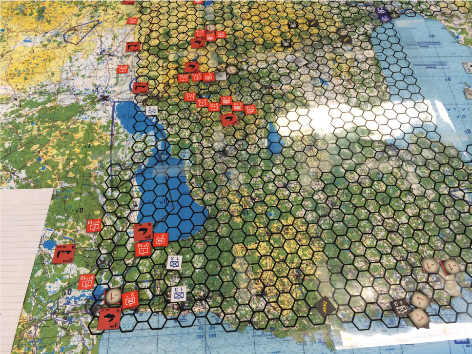


 [This piece was originally posted on 13 July 2016.]