[The article below is reprinted from April 1997 edition of The International TNDM Newsletter.]
The First Test of the TNDM Battalion-Level Validations: Predicting the Winners
by Christopher A. Lawrence
Part I
In the basic concept of the TNDM battalion-level validation, we decided to collect data from battles from three periods: WWI, WWII, and post-WWII. We then made a TNDM run for each battle exactly as the battle was laid out, with both sides having the same CEV [Combat Effectiveness Value]. The results of that run indicated what the CEV should have been for the battle, and we then made a second run using that CEV. That was all we did. We wanted to make sure that there was no “tweaking” of the model for the validation, so we stuck rigidly to this procedure. We then evaluated each run for its fit in three areas:
- Predicting the winner/loser
- Predicting the casualties
- Predicting the advance rate
We did end up changing two engagements around. We had a similar situation with one WWII engagement (Tenaru River) and one modern period engagement (Bir Gifgafa), where the defender received reinforcements part-way through the battle and counterattacked. In both cases we decided to run them as two separate battles (adding two more battles to our database), with the conditions from the first engagement being the starting strength, plus the reinforcements, for the second engagement. Based on our previous experience with running Goose Green, for all the Falklands Island battles we counted the Milans and Carl Gustavs as infantry weapons. That is the only “tweaking” we did that affected the battle outcome in the model. We also put in a casualty multiplier of 4 for WWI engagements, but that is discussed in the article on casualties.
This is the analysis of the first test, predicting the winner/loser. Basically, if the attacker won historically, we assigned it a value of 1, a draw was 0, and a defender win was -1. In the TNDM results summary, it has a column called “winner” which records either an attacker win, a draw, or a defender win. We compared these two results. If they were the same, this is a “correct” result. If they are “off by one,” this means the model predicted an attacker win or loss, where the actual result was a draw, or the model predicted a draw, where the actual result was a win or loss. If they are “off by two” then the model simply missed and predicted the wrong winner.
The results are (the envelope please….):
 It is hard to determine a good predictability from a bad one. Obviously, the initial WWI prediction of 57% right is not very good, while the Modern second run result of 97% is quite good. What l would really like to do is compare these outputs to some other model (like TACWAR) to see if they get a closer fit. I have reason to believe that they will not do better.
Most cases in which the model was “off by 1″ were easily correctable by accounting for the different personnel capabilities of the army. Therefore, just to look where the model really failed. let‘s just look at where it simply got the wrong winner:
 The TNDM is not designed or tested for WWI battles. It is basically designed to predict combat between 1939 and the present. The total percentages without the WWI data in it are:
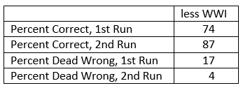 Overall, based upon this data I would be willing to claim that the model can predict the correct winner 75% of the time without accounting for human factors and 90% of the time if it does.
CEVs: Quite simply a user of the TNDM must develop a CEV to get a good prediction. In this particular case, the CEVs were developed from the first run. This means that in the second run, the numbers have been juggled (by changing the CEV) to get a better result. This would make this effort meaningless if the CEVs were not fairly consistent over several engagements for one side versus its other side. Therefore, they are listed below in broad groupings so that the reader can determine if the CEVs appear to be basically valid or are simply being used as a “tweak.”
Now, let’s look where it went wrong. The following battles were not predicted correctly:
 There are 19 night engagements in the data base, five from WWI, three from WWII, and 11 modern. We looked at whether the miss prediction was clustered among night engagements and that did not seem to be the case. Unable to find a pattern, we examined each engagement to see what the problem was. See the attachments at the end of this article for details.
We did obtain CEVs that showed some consistency. These are shown below. The Marines in World War l record the following CEVs in these WWI battles:
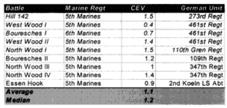 Compare those figures to the performance of the US Army:
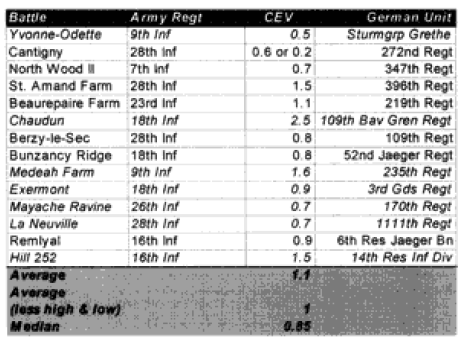 In the above two and in all following cases, the italicized battles are the ones with which we had prediction problems.
For comparison purposes, the CEVs were recorded in the battles in World War II between the US and Japan:
 For comparison purposes, the following CEVs were recorded in Operation Veritable:
 These are the other engagements versus Germans for which CEVs were recorded:
 For comparison purposes, the following CEVs were recorded in the post-WWII battles between Vietnamese forces and their opponents:
 Note that the Americans have an average CEV advantage of 1 .6 over the NVA (only three cases) while having a 1.8 advantage over the VC (6 cases).
For comparison purposes, the following CEVs were recorded in the battles between the British and Argentine’s:






 The December 2018 issue of

 While perusing Charles Shrader’s fascinating