Today’s Friday Read summarizes a series of posts detailing a validation test of the Tactical Numerical Deterministic Model (TNDM) conducted by TDI in 1996. The test was conducted using a database of 76 historical battalion-level combat engagements ranging from World War I through the post-World War II era. It is provided here as an example of how such testing can be done and how useful it can be, despite skepticism expressed by some in the U.S. operations research and modeling and simulation community.
Gun crew from Regimental Headquarters Company, U.S. Army 23rd Infantry Regiment, firing 37mm gun during an advance against German entrenched positions, 1918. [Wikipedia/NARA]
The Second Test of the Battalion-Level Validation: Predicting Casualties Final Scorecard by Christopher A. Lawrence
While writing the article on the use of armor in the Battalion-Level Operations Database (BLODB), I discovered that l had really not completed my article in the last issue on the results of the second battalion-level validation test of the TNDM, casualty predictions. After modifying the engagements for time and fanaticism. I didn’t publish a final “scorecard” of the problem engagements. This became obvious when l needed that scorecard for the article on tanks. So the “scorecards” are published here and are intended to complete the article in the previous issue on predicting casualties.
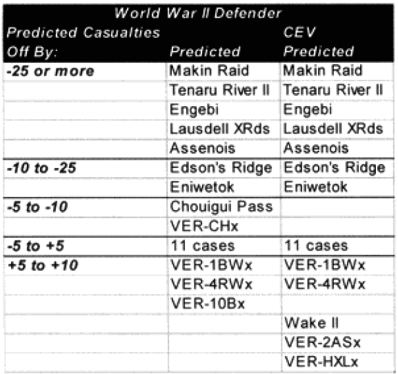
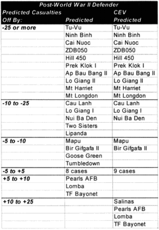
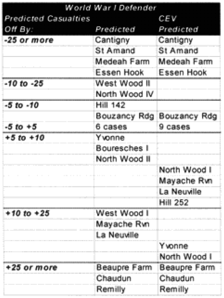
As you certainly recall, amid the 40 graphs and charts were six charts that showed which engagements were “really off.” They showed this for unmodified engagements and CEV modified engagements. We then modified the results of these engagements by the formula for time and “casualty insensitive” systems, we are now listing which engagements were still “off” after making these adjustments.
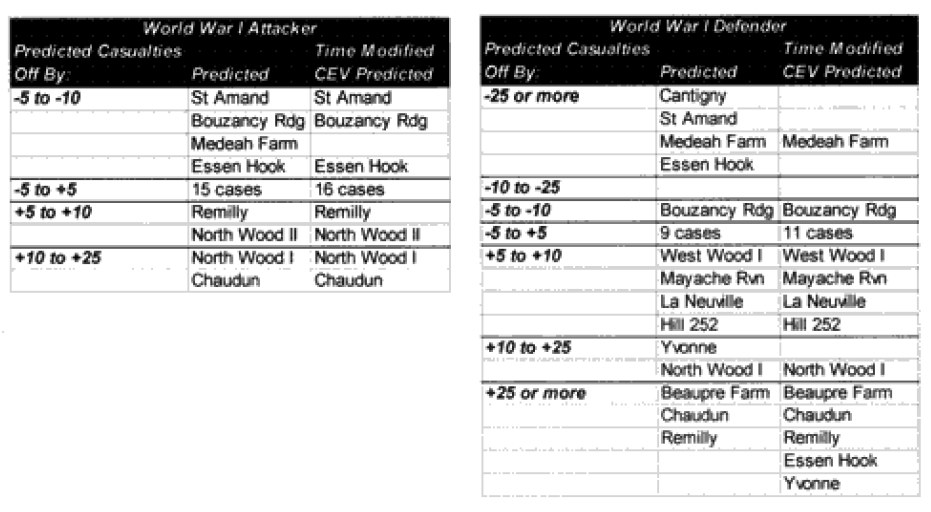
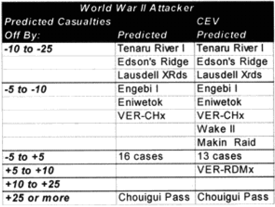
Each table lists how far each engagement was off in gross percent of error. For example, if an engagement like North Wood I had 9.6% losses for the attacker, and the model (with CEV incorporated) predicted 20.57%, then this engagement would be recorded as +10 to +25% off. This was done rather than using a ratio, for having the model predict 2% casualties when there was only 1% is not as bad of an error as having the model predicting 20% when there was only 10%. These would be considered errors of the same order of magnitude if a ratio was used. So below are the six tables.
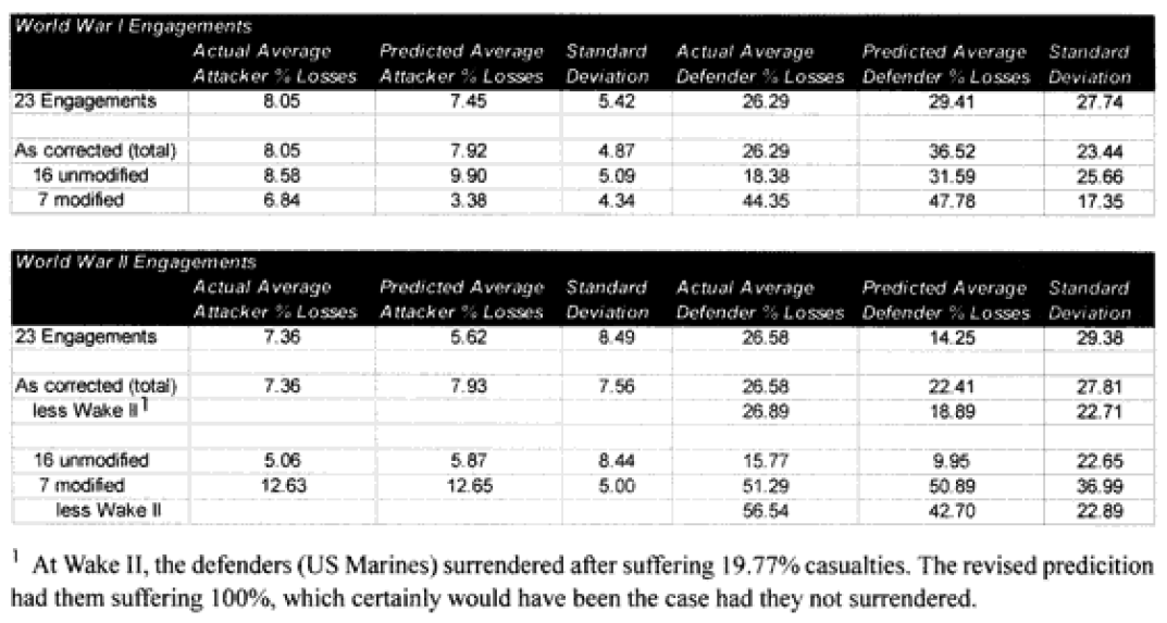
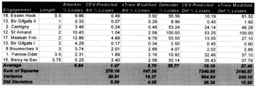
Seven of the World War I battles were modified to account for time. In the case of the attackers we are now getting results with plus or minus 5% in 70% of the cases. In the case of the defenders, we are now getting results of plus or minus 10% in 70% of the cases. As the model doesn’t fit the defender‘s casualties as well as the attacker‘s, I use a different scaling (10% versus 5%) for what is a good fit for the two.
Two cases remain in which the predictions for the attacker are still “really off” (over 10%), while there are six (instead of the previous seven) cases in which the predictions for the defender are “really off” (over 25%).
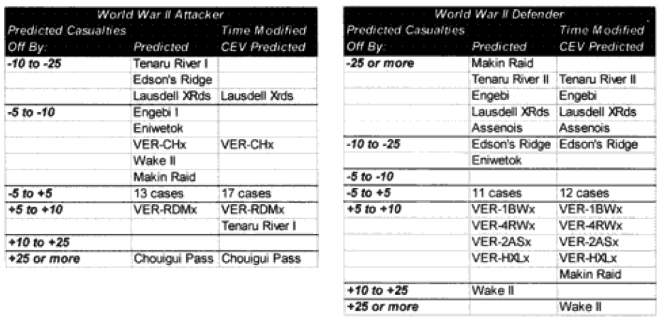
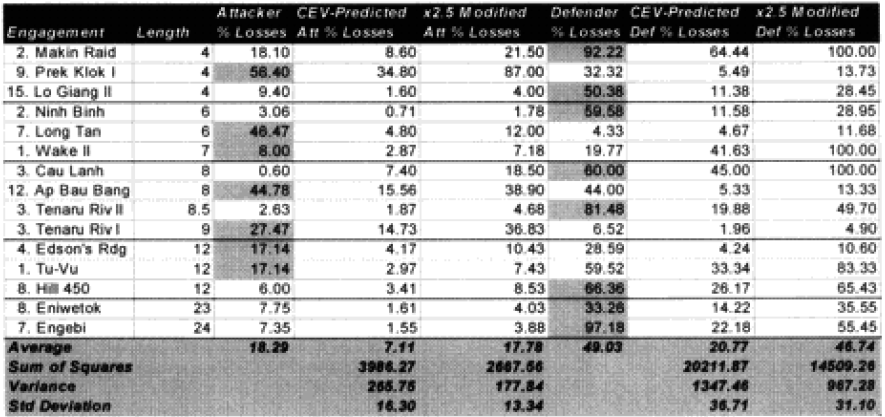
Seven of the World War II battles were modified to account for “casualty insensitive” systems (all Japanese engagements). Time was not an issue in the World War II engagements because all the battles lasted four hours or more. In the case of the attackers, we are now getting results with plus or minus 5% in almost 75% of the cases. In the case of the defenders, we are now getting results of plus or minus 10% in almost 75% of the cases. We are still maintaining the different scaling (5% versus 10%) for what is a good fit for the two.
Now in only two cases (used to be four cases) are the predictions for the attacker really off (over 10%), while there are still five cases in which the predictions for the defender are “really off” (over 25%).
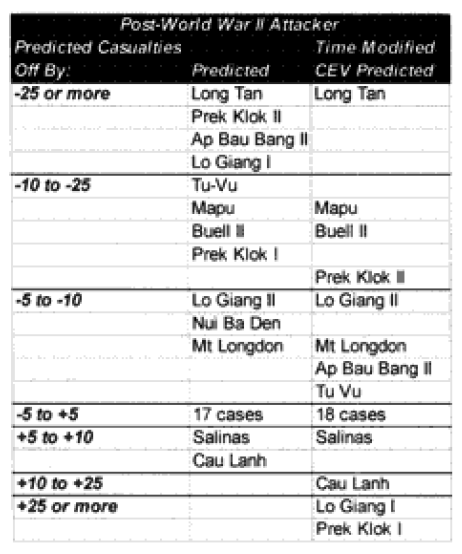
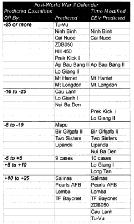
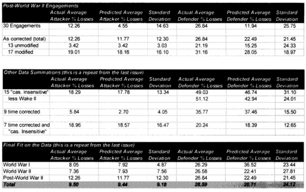
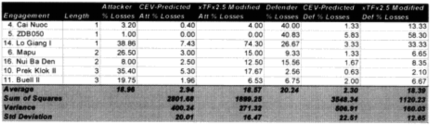
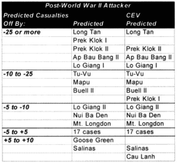
Only 13 of the 30 post-World War II engagements were not changed. Two were modified for time, eight were modified for “casualty insensitive” systems, and seven were modified for both conditions.
In the case of the attackers we are now getting results within plus or minus 5% in 60% of the cases. In the case of the defenders, we are now getting results within plus or minus 10% in around 55% of the cases. We are still maintaining the different scaling (5% versus 10%) for what is a good fit for the two.
We have seven cases (used to be eight cases) in which the attacker‘s predictions are “really off” (over 10%), while there are only five cases (used to be 10) in which the defender‘s casualty predictions are “really off” (over 25%).
Repetitious Conclusion
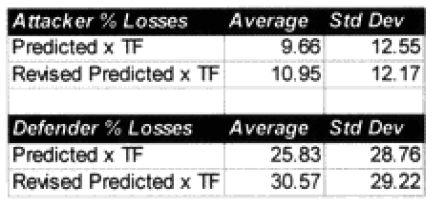
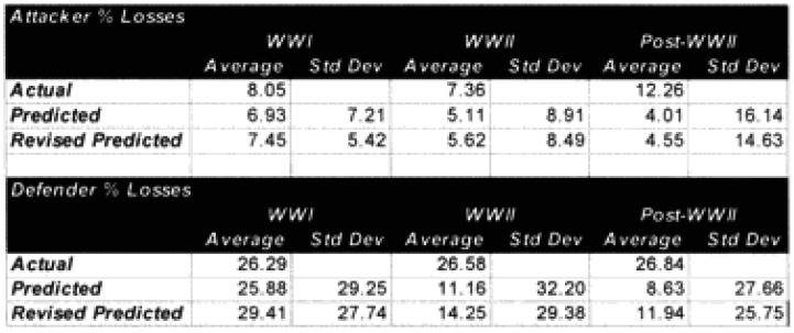
To repeat some of the statistics from the article in the previous issue, in a slightly different format:
The Second Test of the TNDM Battalion-Level Validations: Predicting Casualties by Christopher A. Lawrence
FANATICISM AND CASUALTY INSENSITIVE SYSTEMS:
It was quite clear from looking at the battalion-level data before we did the validation runs that there appeared to be two very different loss patterns, based upon—dare I say it—nationality. See the article in issue 4 of the TNDM Newsletter, “Looking at Casualties Based Upon Nationality Using the BLODB.” While this is clearly the case with the Japanese in WWII, it does appear that other countries were also operating in a manner that produced similar casualty results. So, instead of using the word fanaticism, let’s refer to them as “casualty insensitive” systems. For those who really need a definition before going forward:
“Casualty Insensitive” System: A social or military system that places a high priority on achieving the objective or fulfilling the mission and o low priority on minimizing casualties. Such systems lend to be “mission obsessive” versus using some form of “cost benefit” method of weighing whether the objective is worth the losses suffered to take it.
EXAMPLES OF CASUALTY INSENSITIVE SYSTEMS:
For the purpose of the database, casualty sensitive systems were defined as the Japanese and all highly motivated communist-led armies. These include:
Japanese Army, WWII
Viet Mihn
Viet Cong
North Vietnamese
Indonesian
We have included the Indonesians in this list even though it was based upon only one example.
In the WWII and post-WWII period, one would expect that the following armies would also be “casualty insensitive”
Soviet Army in WWII
North Korean Army
Communist Chinese Army in Korea
Iranian “Pasdaran“
Data can certainly be found to test these candidates.
One could postulate that the WWI attrition multiplier of 4 that we used also incorporates the 2.5 “casualty insensitive” multiplier. This would imply that there was only a multiplier of 1.6 to account for other considerations, like adjusting to the impact of increased firepower on the battlefield. One could also postulate that certain nations, like Russia, have had “casualty insensitive” systems throughout their last 100 years of history. This could also be tested by looking of battles over time of Russians versus Germans compared to Germans versus British, U.S. or French. One could easily carry this analysis back to the Seven Years’ War. If this was the case, this would establish a clear cultural basis for the “casualty insensitive” multiplier, but to do so would require the TNDM to be validated for periods before 1900. This would all be useful analysis in the future, but is not currently budgeted for.
It was expected that the “casualty insensitive” multiplier of 2.5 derived from the Japanese data would be too high to apply directly to the armies. Much to our surprise, we found that this did not appear to be the case. This partially or wholly explained the under-prediction of the 15 of our 20 significantly under-predicted post-WWII engagements. Time would explain another one. And four were not explained.
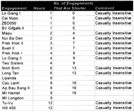
The model noticeably underestimated all the engagements under nine hours except Bir Gifgafa I (2 hours). Pearls AFB (4.5) and Wireless Ridge (8 hours). It noticeably under-estimated all the 15 “fanatic” engagements. If the formulations derived from the earlier data were used here (engagements less than 4 hours and fanatic), then there are 17 engagements in which one side is “casualty insensitive” or in which the engagement time is less than 4 hours. Using the above formulations then 17 engagements would have their casualty figures changed.
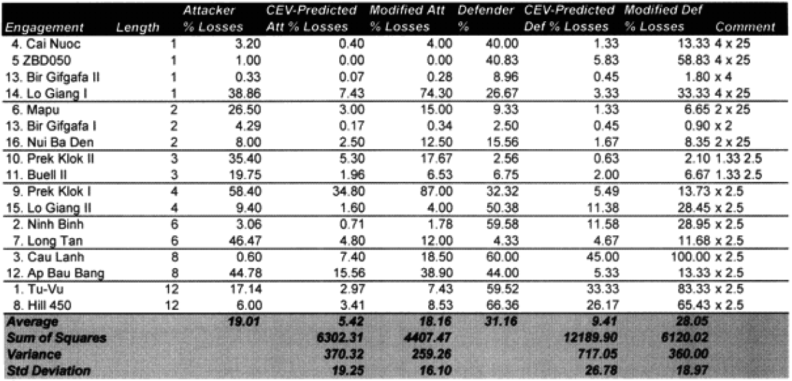
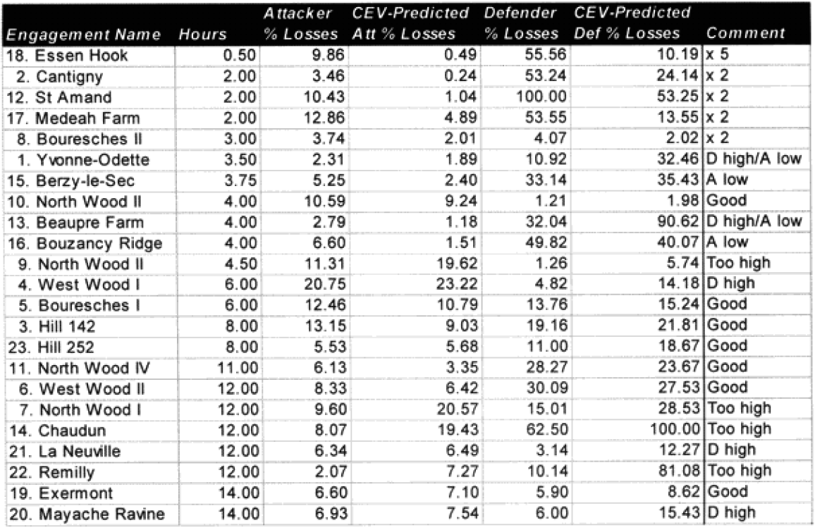
The modified percent loss figures are the CEV predicted percent loss times the factor for “casualty insensitive” systems (for those 15 cases where it applies) and times the formulation for battles less than 4 hours (for those 9 cases where it applies).
Looking at the table at the top of the next page, it would appear that we are on the correct path. But to be safe, on the next page let’s look at the predictive value of the 13 engagements for which we didn’t redefine the attrition multipliers.
The 13 engagements left unchanged:
So, we are definitely heading in the right direction now. We have identified two model changes—time and “casualty insensitive.” We have developed preliminary formulations for time and for “casualty insensitive” forces. Unfortunately, the time formulation was based upon seven WWI engagements. The “casualty insensitive” formulation was based upon seven WWII engagements. Let’s use all our data in the first validation database here for the moment to come up with figures with which we can be more comfortable:
The highlighted entries in the table above indicate “casualty insensitive” forces. We are still struggling with the concept that having one side being casualty insensitive increases both sides’ losses equally. We highlighted them in an attempt to find any other patterns we were missing. We could not.
Now, there may be a more sophisticated measurement of this other than the brute force method of multiplying both sides by 2.5. This might include different multipliers depending on whether one is the fanatic vs non-fanatic side or different multipliers for attack or defense. First, I cannot find any clear indication that there should be a different multiplier for the attacker or defender. A general review of the data confirms that. Therefore, we are saying that the combat relationships between attacker and defender do not change in high intensity or casualty insensitive battles from those experienced in the norm.
What is also clear is that our multiplier of 2.5 appears to be about as good a fit as we can get from a straight multiplier. It does not appear that there is any significant difference between the attrition multiplier for types of “casualty insensitive” systems, whether they are done because of worship of the emperor or because the commissar will shoot slackers. Apparently the mode of fighting is more significant for measuring combat results than how one gets there, although certainly having everyone worship the emperor is probably easier to “administer.”
This still leaves us having to look at whether we should develop a better formulation for time.
Non-fanatic engagement of less than 4 hours:
For fairly obvious reasons, we are still concerned about this formulation for battles of less than one hour, as we have only one example, but until we conduct the second validation, this formulation will remain as is.
Now the extreme cases:
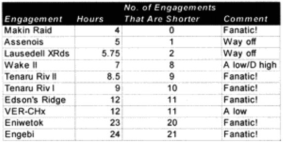
List of all engagements less than 4 hours where one side was fanatic:
It would appear that these formulations of time and “casualty insensitivity” have passed their initial hypothesis formulations tests. We are now willing to make changes to the model based upon this and run the engagements from the second validation data base to test it.
Dead Japanese soldiers lie on the sandbar at the mouth of Alligator Creek on Guadalcanal on 21 August 1942 after being killed by U.S. Marines during the Battle of the Tenaru. [Wikipedia][The article below is reprinted from April 1997 edition of The International TNDM Newsletter.]
The Second Test of the TNDM Battalion-Level Validations: Predicting Casualties by Christopher A. Lawrence
SO WHERE WERE WE REALLY OFF? (WWII)
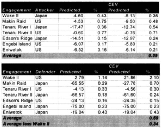
In the ease of the WWII results, we were getting results in the ball park in less than 60% of the cases for the attacker and in less than 50% of the eases in the case of the defenders. We were often significantly too low. Knowing that we were dealing with a number of Japanese engagements (seven), and they clearly fought in a manner that was different from most western European nations, we expected that they would be under-predicting, and some casualty adjustment would be necessary to reflect this.
We also examined whether time was an issue (it was not). The under-predicted battles are listed in the next table
We temporarily defined the Japanese mode of fighting as “fanaticism.” We decided to find a factor for fanaticism by looking at all the battles with the Japanese. They are listed below:
Looking at what multiplier was needed, one notes that .39 times 2.5 = .975 while .34 times 2.5 = .85. This argues for a “fanatic” multiplier of 2.5. The non-fanatic opponent attrition multiplier is also 2.5. There was no indication that both sides should not be affected by the same multiplier.
We had now tentatively identified two “fixes” to the data. l am sure someone will call them “fudges,“ but I am comfortable enough with the logic behind them (especially the fanaticism) that I would dismiss such criticism. It was now time to look at the modern data, and see what would happen if these fixes were applied to it.
SO WHERE WERE WE REALLY OFF? (Post-WWII)
A total of 20 battles were noticeably under-predicted. We examined them to see if there was a pattern in this under-prediction.
The Second Test of the TNDM Battalion-Level Validations: Predicting Casualties by Christopher A. Lawrence
TIME AND THE TNDM:
Before this validation was even begun, I knew we were going to have a problem with the fact that most of the engagements were well below 24 hours in length. This problem was discussed in depth in “Time and the TNDM,” in Volume l, Number 3 of this newsletter. The TNDM considers the casualties for an engagement of less than 24 hours to be reduced in direct proportion to that time. I postulated that the relationship was geometric and came up with a formulation that used the square root of that fraction (i.e. instead of 12 hours being .5 times casualties. it was now .75 times casualties). Being wedded to this idea, l tested this formulation in all ways and for several days, I really wasn’t getting a better fit. All I really did was multiply all the points so that the predicted average was closer. The top-level statistics were:
TF=Time Factor
I also looked out how the losses matched up by one of three periods (WWI, WWII. and post-WWII). When we used the time factor multiplier for the attackers, the WWI engagements average became too high, and the standard deviation increase, same with WWII, while the post-WWII averages were still too low, but the standard deviations got better. For the defender, we got pretty much the same pattern, except now the WWII battles were under-predicting, but the standard deviation was about the same. It was quite clear that all I had with this time factor was noise.
Like any good chef, my failed experiment went right down the disposal. This formulation died a natural death. But looking by period where the model was doing well, and where it wasn’t doing well is pretty telling. The results were:
Looking at the basic results. I could see that the model was doing just fine in predicting WWI battles, although its standard deviation for the defenders was still poor. It wasn’t doing very well with WWII, and performed quite poorly with modem engagements. This was the exact opposite effect to our test on predicting winners and losers, where the model did best with the post-WWII battles and worst with the WWI battles. Recall that we implemented an attrition multiplier of 4 for the WWI battles. So it was now time to look at each battle, and figure out where were we really off. In this case. I looked at casualty figures that were off by a significant order of magnitude. The reason l looked at significant orders of magnitude instead of percent error, is that making a mistake like predicting 2% instead of 1% is not a very big error, whereas predicting 20%, and having the actual casualties 10%, is pretty significant. Both would be off by 100%.
SO WHERE WERE WE REALLY OFF? (WWI)
In the case of the attackers, we were getting a result in the ball park in two-thirds of the cases, and only two cases—N Wood 1 and Chaudun—were really off. Unfortunately, for the defenders we were getting a reasonable result in only 40% of the cases, and the model had a tendency to under-or over-predict.
It is clear that the model understands attacker losses better than defender losses. I suspect this is related to the model having no breakpoint methodology. Also, defender losses may be more variable. I was unable to find a satisfactory explanation for the variation. One thing I did notice was that all four battles that were significantly under-predicted on the defender sides were the four shortest WWI battles. Three of these were also noticeably under-predicted for the attacker. Therefore. I looked at all 23 WWI engagements related to time.
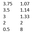
Looking back at the issue of time, it became clear the model was clearly under-predicting in battles of less than four hours. I therefore came up with the following time scaling formula:
If time of battle less than four hours, then multiply attrition by (4/(Length of battle in hours)).
What this formula does is make all battles less than four hours equal to a four-hour engagement. This intuitively looks wrong, but one must consider how we define a battle. A “battle” is defined by the analyst after the fact. The start time is usually determined by when the attack starts (or when the artillery bombardment starts) and end time by when the attack has clearly failed, or the mission has been accomplished, or the fighting has died down. Therefore, a battle is not defined by time, but by resolution.
As such, any battle that only lasts a short time will still have a resolution, and as a result of achieving that resolution there will be considerable combat experience. Therefore, a minimum casualty multiplier of 1/6 must be applied to account for that resolution. We shall see if this is really the case when we run the second validation using the new battles, which have a considerable number of brief engagements. For now, this seems to fit.
As for all the other missed predictions, including the over-predictions, l could not find a magic formula that connected them. My suspicion was that the multiplier of x4 would be a little too robust, but even after adjusting for the time equation, this left 14 of the attacker‘s losses under-predicted and six of the defender actions under-predicted. If the model is doing anything, it is under-predicting attacker casualties and over-predicting defender casualties. This would argue for a different multiplier for the attacker than for the defender (higher one for the attacker). We had six cases where the attacker‘s and defenders predictions were both low, nine where they were both high, and eight cases where the attackers prediction was low while the defender’s prediction was high. We had no cases where the attacker’s prediction was high and the defender’s prediction was low. As all these examples were from the western front in 1918, U.S. versus Germans, then the problem could also be that the model is under-predicting the effects of fortifications, or the terrain for the defense. It could also be indicative of a fundamental difference in the period that gave the attackers higher casualty rates than the defenders. This is an issue I would like to explore in more depth, and l may do so after l have more WWI data from the second validation.
The Second Test of the TNDM Battalion-Level Validations: Predicting Casualties by Christopher A. Lawrence
Actually, l was pretty pleased with the first test of the TNDM, predicting winners and losers. I wasn’t too pleased with how it did with WWI, but was quite pleased with its prediction of post-WWII combat. But l knew from our previous analysis that we were going to have some problems with the casualty prediction estimates for WWI, for any battles that the Japanese were involved with, and for shorter engagements.
For period 1900-1945. Russian and Japanese rates are double those calculated.
For period 1914-1941, rates as calculated must be doubled; for Russian, Turkish, and Balkan forces they must be quadrupled.
For 1950-1953 rate as calculated will apply for UN forces (other than ROK): for ROK. North Koreans, and Chinese rates are doubled.
The attrition calculation for the TNDM is different from that used in the QJM. Actually the attrition calculations for the later versions of the QJM differ from the earlier versions. The base casualty rates that are used in the original QJM are very different from those used in the TNDM. See my articles in the TNDM Newsletter, Volume 1, Issue 3. Basically the QJM starts with a based factor of 2.8% for attackers versus 4% for the TNDM, while its base factor for defenders is 1.5% versus 6% for the TNDM.
When Dave Bongard did the first TNDM runs for this validation effort, he automatically added in an attrition multiplier of 4 for all the WWI battles. This undocumented methodology was implemented by Mr. Bongard instinctively because he knew from experience that you need to multiply the attrition rates by 4 for WWI battles. I decided to let it stand and see how it measured up during the validation.
We then made our two model runs for each validation, first without the CEV, and a second run with the CEV incorporated. I believe the CEV results from this methodology are explained in the previous article on winners and losers.
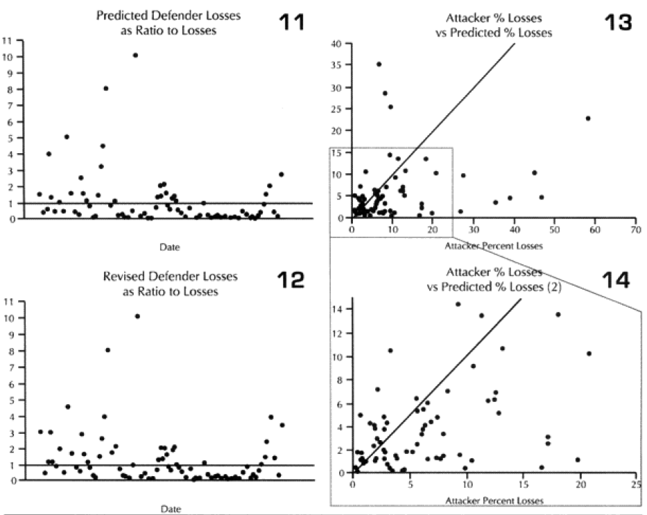
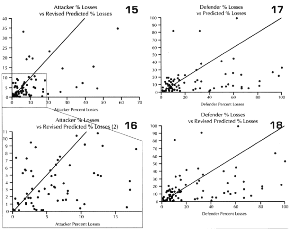
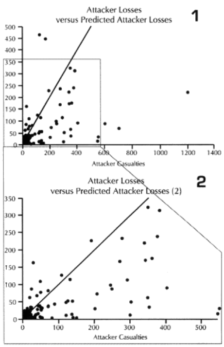
At the top of the next column is a comparison of the attacker losses versus the losses predicted by the model (graphs 1 and 2). This is in two scales, so you can see the details of the data.
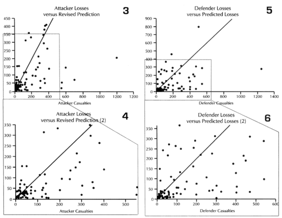
The diagonal line across these graphs and across the next seven graphs is the “perfect prediction” line, with any point on that line being perfectly predicted. The closer a point is to that line, the better the prediction. Points to the left of that line is where the model over-predicted casualties, while the points to the right is where the model under-predicted. We also ran the model using the CEV as predicted by the model. This “revised prediction” is shown in the next graph (see graphs 3 and 4). We also have done the same comparison of total casualties for the defender (see graphs 5 through 8).
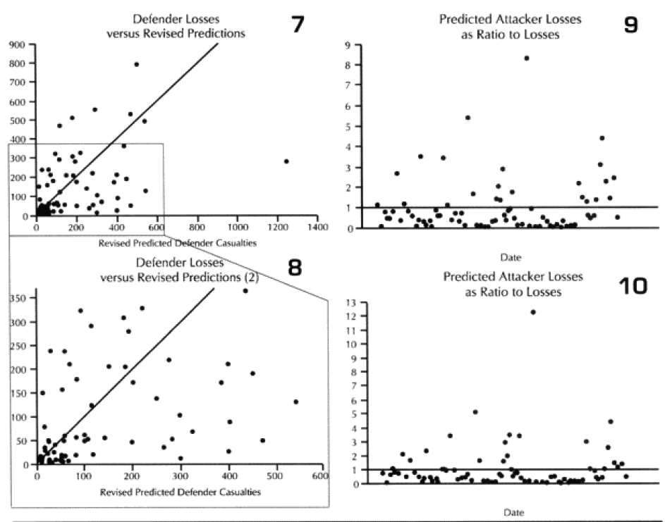
The model is clearly showing a tendency to under-predict. This is shown in the next set of graphs, where we divided the predicted casualties by the actual casualties. Values less than one are under-predictions. That means everything below the horizontal line shown on the graph (graph 9) is under-predicted. The same tests were done the “revised prediction“ (meaning with CEV) for the attacker and the both predictions for the defender (graphs 10-12).
I then attempted to do some work using the total casualty figures, followed by a series of meaningless tests of the data based upon force size. Force sizes range widely, and the size of forces committed to battle has a significant impact on the total losses. Therefore, to get anything useful, l really needed to look at percent of losses, not gross losses. These are displayed in the next 6 graphs (graphs 13-18).
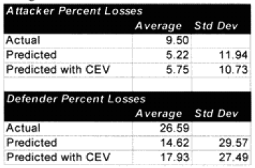
Comparing our two outputs (model prediction without CEV incorporated and model prediction with CEV incorporated) to the 76 historical engagements gives the following disappointing results:
The standard deviation was measured by taking each predicted result, subtracting from it the actual result squaring it, summing all 76 cases, dividing by 76, and taking the square root. (see sidebar A Little Basic Statistics below.)
First and foremost, the model was under-predicting by a factor of almost two. Furthermore it was running high standard deviations. This last result did not surprise me considering the nature of the battalion-level combat.
The addition of the CEVs did not significantly change the casualties. This is because in the attrition equations, the conditions of the battlefield play an important part in determining casualties. People in the past have claimed that the CEVs were some type of fudge factor. If that is the case, then it is a damned lousy fudge factor. If the TNDM is getting a good prediction on casualties, it is not because of a CEV “fudge factor.”
SIDEBAR: A Little Basic Statistics
The mean is 5.75 for the attacker and 17.93 for the defender, the standard deviation is 10.73 for the attacker and 27.49 for the defender. The number of examples is 76, the degree of freedom is 75. Therefore the confidence intervals are:
With the actual average being 9.50, we are clearly predicting too low.
With the actual average being 26.59, we are again clearly predicting too low.
The First Test of the TNDM Battalion-Level Validations: Predicting the Winners by Christopher A. Lawrence
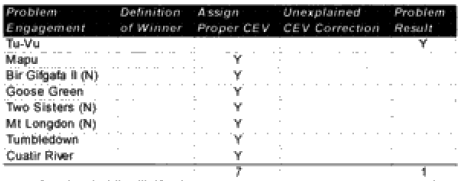
CASE STUDIES: WHERE AND WHY THE MODEL FAILED CORRECT PREDICTIONS
Modern (8 cases):
Tu-Vu—On the first run, the model predicted a defender win. Historically, the attackers (Viet Minh) won with a 2.8 km advance. When the CEV for the Viet Minh was put in (1.2), the defender still won. The real problem in this case is the horrendous casualties taken by both sides, with the defending Moroccans losing 250 out of 420 people and the attacker losing 1,200 out of 7,000 people. The model predicted only 140 and 208 respectively. This appears to address a fundamental weakness in the model, which is that if one side is willing to attack (or defend) at all costs, the model cannot predict the extreme losses. This happens in some battles with non-first world armies, with the Japanese in WWII, and apparently sometimes with the WWI predictions. In effect, the model needs some mechanism to predict fanaticism that would increase the intensity and casualties of the battle for both sides. In this case, the increased casualties certainly would have resulted in an attacker advance after over half of the defenders were casualties.
Mapu—On the first run the model predicted an attacker (Indonesian) win. Historically, the defender (British) won. When the British are given a hefty CEV of 2.6 (as one would expect that they would have), the defender wins, although the casualties are way off for the attacker. This appears to be a case in which the side that would be expected to have the higher CEV needed that CEV input into the combat run.
Bir Gifgafa II (Night)—On the first run the model predicted a defender (Egyptian) win. Historically the attacker (Israel) won with an advance of three kilometers. When the Israelis are given a hefty CEV of 3.5 (as historically they have tended to have), they win, although their casualties and distance advanced are way off. These errors are probably due to the short duration (one hour) of the model run. This appears to be a case where the side that would be expected to have the higher CEV needed that CEV input into the combat run in order to replicate historical results.
Goose Green—On the first run the model predicted a draw. Historically, the attacker (British) won. The first run also included the “cheat” of counting the Milans as regular weapons versus anti-tank. When the British are given a hefty CEV of 2.4 (as one could reasonably expect that they would have) they win, although their advance rate is too slow. Casualty prediction is quite good. This appears to be a case where the side that would be expected to have the higher CEV needed that CEV input into the combat run.
Two Sisters (Night)—On the first run the model predicted a draw. Historically the attacker (British) won yet again. When the British are given a CEV of 1.7 (as one would expect that they would have) the attacker wins, although the advance rate is too slow and the casualties a little low. This appears to be a case where the side that would be expected to have the higher CEV needed that CEV input into the combat run.
Mt. Longdon (Night)—0n the first run the model predicted a defender win. Historically, the attacker (British) won as usual. When the British are given a CEV of 2.3 (as one would expect that they should have) the attacker wins, although as usual the advance rate is too slow and the casualties a little low. This appears to be a case where the side that would be expected to have the higher CEV needed that CEV input into the combat run.
Tumbledown—On the first run the model predicted a defender win. Historically the attacker (British) won as usual. When the British were given a CEV of 1.9 (as one would expect that they should have), the attacker wins, although as usual, the advance rate is too slow and the casualties a little low. This appears to be a case where the side that would be expected to have the higher CEV needed that CEV input into the combat run.
Cuatir River—On the first run the model predicted a draw. Historically, the attacker (The Republic of South Africa) won. When the South African forces were given a CEV of 2.3 (as one would expect that they should have) the attacker wins, with advance rates and casualties being reasonably close. This appears to be a case where the side that would be expected to have the higher CEV needed that CEV input into the combat run.
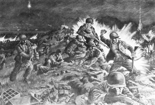
A painting by a Marine officer present during the Guadalcanal campaign depicts Marines defending Hill 123 during the Battle of Edson’s Ridge, 12-14 September 1942. [Wikipedia]
The First Test of the TNDM Battalion-Level Validations: Predicting the Winners by Christopher A. Lawrence
CASE STUDIES: WHERE AND WHY THE MODEL FAILED CORRECT PREDICTIONS
World War ll (8 cases):
Overall, we got a much better prediction rate with WWII combat. We had eight cases where there was a problem. They are:
Makin Raid—On the first run, the model predicted a defender win. Historically, the attackers (US Marines) won with a 2.5 km advance. When the Marine CEV was put in (a hefty 2.4), this produced a reasonable prediction, although the advance rate was too slow. This appears to be a case where the side that would be expected to have the higher CEV needed that CEV input into the combat run in order to replicate historical results.
Edson’s Ridge (Night)—On the first run, the model predicted a defender win. Historically, the battle must be considered at best a draw, or more probably a defender win, as the mission accomplishment score of the attacker is 3 while the defender is 5.5. The attacker did advance 2 kilometers, but suffered heavy casualties. The second run was done with a US CEV of 1.5. This maintained a defender win and even balanced more in favor of the Marines. This is clearly a problem in defining who is the winner.
Lausdell X-Road: (Night)—On the first run, the model predicted an attacker victory with an advance rate of 0.4 kilometer. Historically, the German attackers advanced 0.75 kilometer, but had a mission accomplishment score of 4 versus the defender’s mission accomplishment score of 6. A second run was done with a US CEV of 1.1, but this did not significantly change the result. This is clearly a problem in defining who is the winner.
VER-9CX—On the first run, the attacker is reported as the winner. Historically this is the case, with the attacker advancing 1.2 kilometers although suffering higher losses than the defender. On the second run, however, the model predicted that the engagement was a draw. The model assigned the defenders (German) a CEV of 1.3 relative to the attackers in attempt to better reflect the casualty exchange. The model is clearly having a problem with this engagement due to the low defender casualties.
VER-2ASX—On the first run, the defender was reported as the winner. Historically, the attacker won. On the second run, the battle was recorded as a draw with the attacker (British) CEV being 1.3. This high CEV for the British is not entirely explainable, although they did fire a massive suppressive bombardment. In this case the model appears to be assigning a CEV bonus to the wrong side in an attempt to adjust a problem run. The model is still clearly having a problem with this engagement due to the low defender casualties.
VER-XHLX—On the first run, the model predicted that the defender won. Historically, the attacker won. On the second run, the battle was recorded as an attacker win with the attacker (British) CEV being 1.3. This high CEV is not entirely explainable. There is no clear explanation for these results.
VER-RDMX—On the first run, the model predicted that the attacker won. Historically, this is correct. On the second run, the battle recorded that the defender won. This indicates an attempt by the model to get the casualties correct. The model is clearly having a problem with this engagement due to the low defender casualties.
VER-CHX—On the first run, the model predicted that the defender won. Historically, the attacker won. On the second run, the battle was recorded as an attacker win with the attacker (Canadian) CEV being 1.3. Again, this high CEV is not entirely explainable. The model appears to be assigning a CEV bonus to the wrong side in an attempt to adjust a problem run. The model is still clearly having a problem with this engagement due to the low defender casualties.
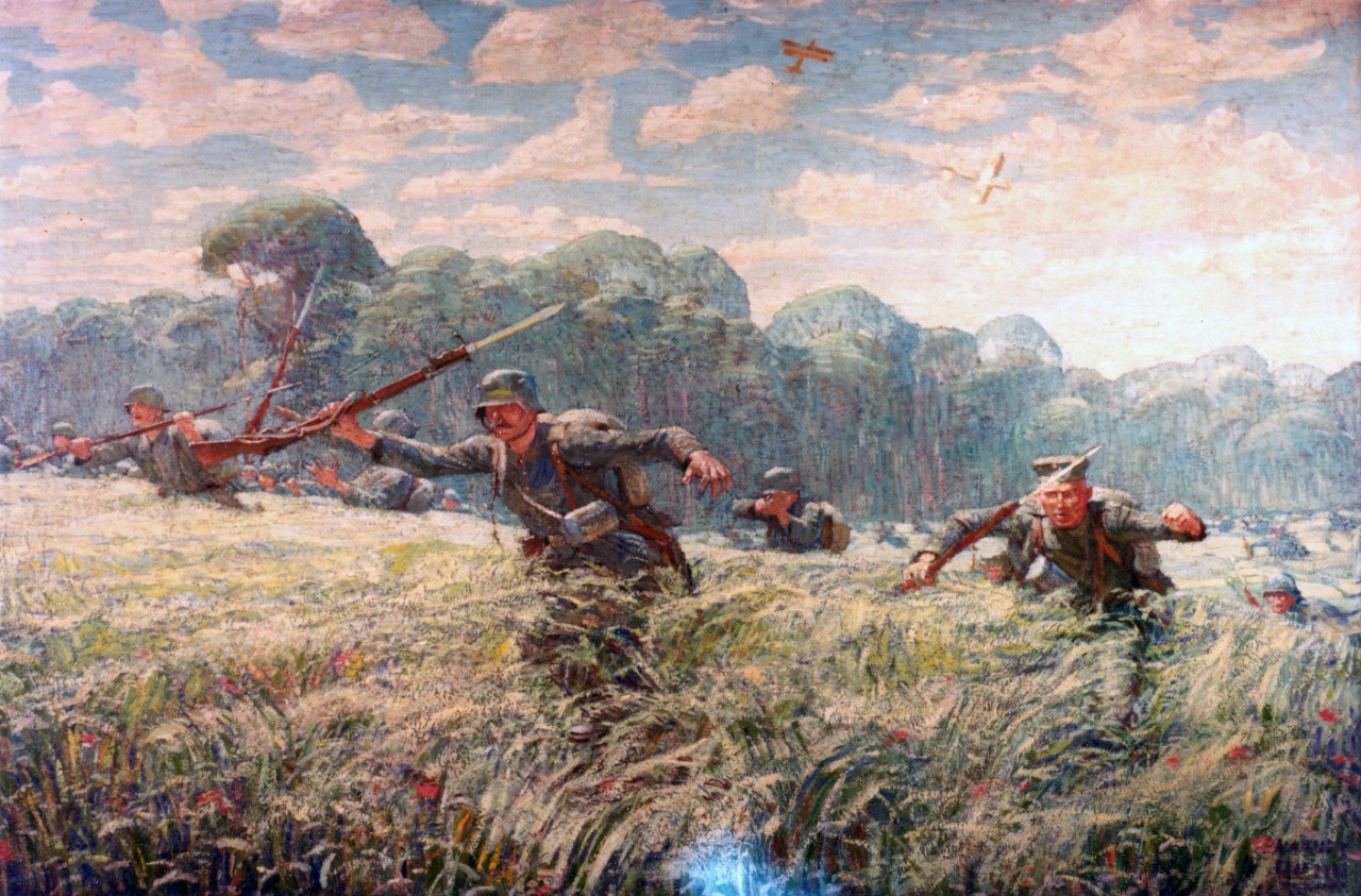
Advancing Germans halted by 2nd Battalion, Fifth Marine, June 3 1918. Les Mares form 2 1/2 miles west of Belleau Wood attacked the American lines through the wheat fields. From a painting by Harvey Dunn. [U.S. Navy]
The First Test of the TNDM Battalion-Level Validations: Predicting the Winners by Christopher A. Lawrence
CASE STUDIES: WHERE AND WHY THE MODEL FAILED CORRECT PREDICTIONS
World War I (12 cases):
Yvonne-Odette (Night)—On the first prediction, selected the defender as a winner, with the attacker making no advance. The force ratio was 0.5 to 1. The historical results also show e attacker making no advance, but rate the attacker’s mission accomplishment score as 6 while the defender is rated 4. Therefore, this battle was scored as a draw.
On the second run, the Germans (Sturmgruppe Grethe) were assigned a CEV of 1.9 relative to the US 9th Infantry Regiment. This produced a draw with no advance.
This appears to be a result that was corrected by assigning the CEV to the side that would be expected to have that advantage. There is also a problem in defining who is winner.
Hill 142—On the first prediction the defending Germans won, whereas in the real world the attacking Marines won. The Marines are recorded as having a higher CEV in a number of battles, so when this correction is put in the Marines win with a CEV of 1.5. This appears to be a case where the side that would be expected to have the higher CEV needed that CEV input into the combat rim to replicate historical results.
Note that while many people would expect the Germans to have the higher CEV, at this juncture in WWI the German regular army was becoming demoralized, while the US Army was highly motivated, trained and fresh. While l did not initially expect to see a superior CEV for the US Marines, when l did see it l was not surprised. I also was not surprised to note that the US Army had a lower CEV than the Marine Corps or that the German Sturmgruppe Grethe had a higher CEV than the US side. As shown in the charts below, the US Marines’ CEV is usually higher than the German CEV for the engagements of Belleau Wood, although this result is not very consistent in value. But this higher value does track with Marine Corps legend. l personally do not have sufficient expertise on WWI to confirm or deny the validity of the legend.
West Wood I—0n the first prediction the model rated the battle a draw with minimal advance (0.265 km) for the attacker, whereas historically the attackers were stopped cold with a bloody repulse. The second run predicted a very high CEV of 2.3 for the Germans, who stopped the attackers with a bloody repulse. The results are not easily explainable.
Bouresches I (Night)—On the first prediction the model recorded an attacker victory with an advance of 0.5 kilometer. Historically, the battle was a draw with an attacker advance of one kilometer. The attacker’s mission accomplishment score was 5, while the defender’s was 6. Historically, this battle could also have been considered an attacker victory. A second run with an increased German CEV to 1.5 records it as a draw with no advance. This appears to be a problem in defining who is the winner.
West Wood II—On the first run, the model predicted a draw with an advance of 0.3 kilometers. Historically, the attackers won and advanced 1.6 kilometers. A second run with a US CEV of 1.4 produced a clear attacker victory. This appears to be a case where the side that would be expected to have the higher CEV needed that CEV input into the combat run.
North Woods I—On the first prediction, the model records the defender winning, while historically the attacker won. A second run with a US CEV of 1.5 produced a clear attacker victory. This appears to be a case where the side that would be expected to have the higher CEV needed that CEV input into the combat run.
Chaudun—On the first prediction, the model predicted the defender winning when historically, the attacker clearly won. A second run with an outrageously high US CEV of 2.5 produced a clear attacker victory. The results are not easily explainable.
Medeah Farm—On the first prediction, the model recorded the defender as winning when historically the attacker won with high casualties. The battle consists of a small number of German defenders with lots of artillery defending against a large number of US attackers with little artillery. On the second run, even with a US CEV of 1.6, the German defender won. The model was unable to select a CEV that would get a correct final result yet reflect the correct casualties. The model is clearly having a problem with this engagement.
Exermont—On the first prediction, the model recorded the defender as winning when historically, the attacker did, with both the attackers and the defender’s mission accomplishment scores being rated at 5. The model did rate the defender‘s casualties too high, so when it calculated what the CEV should be, it gave the defender a higher CEV so that it could bring down the defenders losses relative to the attackers. Otherwise, this is a normal battle. The second prediction was no better. The model is clearly having a problem with this engagement due to the low defender casualties.
Mayache Ravine—The model predicted the winner (the attacker) correctly on the first run, with the attacker having an opposed advance of 0.8 kilometer. Historically, the attacker had an opposed rate of advance of 1.3 kilometers. Both sides had a mission accomplishment score of 5. The problem is that the model predicted higher defender casualties than the attacker, while in the actual battle the defender had lower casualties that the attacker. On the second run, therefore, the model put in a German CEV of 1.5, which resulted in a draw with the attacker advancing 0.3 kilometers. This brought the casualty estimates more in line, but turned a successful win/loss prediction into one that was “off by one.” The model is clearly having a problem with this engagement due to the low defender casualties.
La Neuville—The model also predicted the winner (the attacker) correctly here, with the attacker advancing 0.5 kilometer. In the historical battle they advanced 1.6 kilometers. But again, the model predicted lower attacker losses than the defender losses, while in the actual battle the defender losses were much lower than the attacker losses. So, again on the second run, the model gave the defender (the Germans) a CEV of 1.4, which turned an accurate win/loss prediction into an inaccurate one. It still didn’t do a very good job on the casualties. The model is clearly having a problem with this engagement due to the low defender casualties.
Hill 252—On the first run, the model predicts a draw with a distanced advanced of 0.2 km, while the real battle was an attacker victory with an advance of 2.9 kilometers. The model’s casualty predictions are quite good. On the second run, the model correctly predicted an attacker win with a US CEV of 1.5. The distance advanced increases to 0.6 kilometer, while the casualty prediction degrades noticeably. The model is having some problems with this engagement that are not really explainable, but the results are not far off the mark.
The First Test of the TNDM Battalion-Level Validations: Predicting the Winners by Christopher A. Lawrence
Part II
CONCLUSIONS:
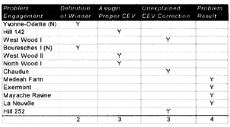
WWI (12 cases):
For the WWI battles, the nature of the prediction problems are summarized as:
CONCLUSION: In the case of the WWI runs, five of the problem engagements were due to confusion of defining a winner or a clear CEV existing for a side that should have been predictable. Seven out of the 23 runs have some problems, with three problems resolving themselves by assigning a CEV value to a side that may not have deserved it. One (Medeah Farm) was just off any way you look at it, and three suffered a problems because historically the defenders (Germans) suffered surprisingly low losses. Two had the battle outcome predicted correctly on the first run, and then had the outcome incorrectly predicted after a CEV was assigned.
With 5 to 7 clear failures (depending on how you count them), this leads one to conclude that the TNDM can be relied upon to predict the winner in a WWI battalion-level battle in about 70% of the cases.
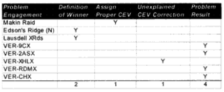
WWII (8 cases):
For the WWII battles, the nature of the prediction problems are summarized as:
CONCLUSION: In the case of the WWII runs, three of the problem engagements were due to confusion of defining a winner or a clear CEV existing for a side that should have been predictable. Four out of the 23 runs suffered a problem because historically the defenders (Germans) suffered surprisingly low losses and one case just simply assigned a possible unjustifiable CEV. This led to the battle outcome being predicted correctly on the first run, then incorrectly predicted after CEV was assigned.
With 3 to 5 clear failures, one can conclude that the TNDM can be relied upon to predict the winner in a WWII battalion-level battle in about 80% of the cases.
Modern (8 cases):
For the post-WWll battles, the nature of the prediction problems are summarized as:
CONCLUSION: ln the case of the modem runs, only one result was a problem. In the other seven cases, when the force with superior training is given a reasonable CEV (usually around 2), then the correct outcome is achieved. With only one clear failure, one can conclude that the TNDM can be relied upon to predict the winner in a modern battalion-level battle in over 90% of the cases.
FINAL CONCLUSIONS: In this article, the predictive ability of the model was examined only for its ability to predict the winner/loser. We did not look at the accuracy of the casualty predictions or the accuracy of the rates of advance. That will be done in the next two articles. Nonetheless, we could not help but notice some trends.
First and foremost, while the model was expected to be a reasonably good predictor of WWII combat, it did even better for modem combat. It was noticeably weaker for WWI combat. In the case of the WWI data, all attrition figures were multiplied by 4 ahead of time because we knew that there would be a fit problem otherwise.
This would strongly imply that there were more significant changes to warfare between 1918 and 1939 than between 1939 and 1989.
Secondly, the model is a pretty good predictor of winner and loser in WWII and modern cases. Overall, the model predicted the winner in 68% of the cases on the first run and in 84% of the cases in the run incorporating CEV. While its predictive powers were not perfect, there were 13 cases where it just wasn’t getting a good result (17%). Over half of these were from WWI, only one from the modern period.
In some of these battles it was pretty obvious who was going to win. Therefore, the model needed to do a step better than 50% to be even considered. Historically, in 51 out of 76 cases (67%). the larger side in the battle was the winner. One could predict the winner/loser with a reasonable degree of success by just looking at that rule. But the percentage of the time the larger side won varied widely with the period. In WWI the larger side won 74% of the time. In WWII it was 87%. In the modern period it was a counter-intuitive 47% of the time, yet the model was best at selecting the winner in the modern period.
The model’s ability to predict WWI battles is still questionable. It obviously does a pretty good job with WWII battles and appears to be doing an excellent job in the modern period. We suspect that the difference in prediction rates between WWII and the modern period is caused by the selection of battles, not by any inherit ability of the model.
RECOMMENDED CHANGES: While it is too early to settle upon a model improvement program, just looking at the problems of winning and losing, and the ancillary data to that, leads me to three corrections:
Adjust for times of less than 24 hours. Create a formula so that battles of six hours in length are not 1/4 the casualties of a 24-hour battle, but something greater than that (possibly the square root of time). This adjustment should affect both casualties and advance rates.
Adjust advance rates for smaller unit: to account for the fact that smaller units move faster than larger units.
Adjust for fanaticism to account for those armies that continue to fight after most people would have accepted the result, driving up casualties for both sides.
 Today’s Friday Read summarizes a series of posts detailing a validation test of the Tactical Numerical Deterministic Model (TNDM) conducted by TDI in 1996. The test was conducted using a database of 76 historical battalion-level combat engagements ranging from World War I through the post-World War II era. It is provided here as an example of how such testing can be done and how useful it can be, despite skepticism expressed by some in the U.S. operations research and modeling and simulation community.