Mystics & Statistics

[The article below is reprinted from April 1997 edition of The International TNDM Newsletter.]

The First Test of the TNDM Battalion-Level Validations: Predicting the Winners
by Christopher A. Lawrence

CASE STUDIES: WHERE AND WHY THE MODEL FAILED CORRECT PREDICTIONS

Modern (8 cases):

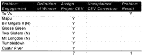
Tu-Vu—On the first run, the model predicted a defender win. Historically, the attackers (Viet Minh) won with a 2.8 km advance. When the CEV for the Viet Minh was put in (1.2), the defender still won. The real problem in this case is the horrendous casualties taken by both sides, with the defending Moroccans losing 250 out of 420 people and the attacker losing 1,200 out of 7,000 people. The model predicted only 140 and 208 respectively. This appears to address a fundamental weakness in the model, which is that if one side is willing to attack (or defend) at all costs, the model cannot predict the extreme losses. This happens in some battles with non-first world armies, with the Japanese in WWII, and apparently sometimes with the WWI predictions. In effect, the model needs some mechanism to predict fanaticism that would increase the intensity and casualties of the battle for both sides. In this case, the increased casualties certainly would have resulted in an attacker advance after over half of the defenders were casualties.

Mapu—On the first run the model predicted an attacker (Indonesian) win. Historically, the defender (British) won. When the British are given a hefty CEV of 2.6 (as one would expect that they would have), the defender wins, although the casualties are way off for the attacker. This appears to be a case in which the side that would be expected to have the higher CEV needed that CEV input into the combat run.

Bir Gifgafa II (Night)—On the first run the model predicted a defender (Egyptian) win. Historically the attacker (Israel) won with an advance of three kilometers. When the Israelis are given a hefty CEV of 3.5 (as historically they have tended to have), they win, although their casualties and distance advanced are way off. These errors are probably due to the short duration (one hour) of the model run. This appears to be a case where the side that would be expected to have the higher CEV needed that CEV input into the combat run in order to replicate historical results.

Goose Green—On the first run the model predicted a draw. Historically, the attacker (British) won. The first run also included the “cheat” of counting the Milans as regular weapons versus anti-tank. When the British are given a hefty CEV of 2.4 (as one could reasonably expect that they would have) they win, although their advance rate is too slow. Casualty prediction is quite good. This appears to be a case where the side that would be expected to have the higher CEV needed that CEV input into the combat run.

Two Sisters (Night)—On the first run the model predicted a draw. Historically the attacker (British) won yet again. When the British are given a CEV of 1.7 (as one would expect that they would have) the attacker wins, although the advance rate is too slow and the casualties a little low. This appears to be a case where the side that would be expected to have the higher CEV needed that CEV input into the combat run.

Mt. Longdon (Night)—0n the first run the model predicted a defender win. Historically, the attacker (British) won as usual. When the British are given a CEV of 2.3 (as one would expect that they should have) the attacker wins, although as usual the advance rate is too slow and the casualties a little low. This appears to be a case where the side that would be expected to have the higher CEV needed that CEV input into the combat run.

Tumbledown—On the first run the model predicted a defender win. Historically the attacker (British) won as usual. When the British were given a CEV of 1.9 (as one would expect that they should have), the attacker wins, although as usual, the advance rate is too slow and the casualties a little low. This appears to be a case where the side that would be expected to have the higher CEV needed that CEV input into the combat run.

Cuatir River—On the first run the model predicted a draw. Historically, the attacker (The Republic of South Africa) won. When the South African forces were given a CEV of 2.3 (as one would expect that they should have) the attacker wins, with advance rates and casualties being reasonably close. This appears to be a case where the side that would be expected to have the higher CEV needed that CEV input into the combat run.

Next: Predicting casualties.

[The article below is reprinted from April 1997 edition of The International TNDM Newsletter.]

The First Test of the TNDM Battalion-Level Validations: Predicting the Winners
by Christopher A. Lawrence

CASE STUDIES: WHERE AND WHY THE MODEL FAILED CORRECT PREDICTIONS

World War ll (8 cases):

Overall, we got a much better prediction rate with WWII combat. We had eight cases where there was a problem. They are:

Makin Raid—On the first run, the model predicted a defender win. Historically, the attackers (US Marines) won with a 2.5 km advance. When the Marine CEV was put in (a hefty 2.4), this produced a reasonable prediction, although the advance rate was too slow. This appears to be a case where the side that would be expected to have the higher CEV needed that CEV input into the combat run in order to replicate historical results.

Edson’s Ridge (Night)—On the first run, the model predicted a defender win. Historically, the battle must be considered at best a draw, or more probably a defender win, as the mission accomplishment score of the attacker is 3 while the defender is 5.5. The attacker did advance 2 kilometers, but suffered heavy casualties. The second run was done with a US CEV of 1.5. This maintained a defender win and even balanced more in favor of the Marines. This is clearly a problem in defining who is the winner.

Lausdell X-Road: (Night)—On the first run, the model predicted an attacker victory with an advance rate of 0.4 kilometer. Historically, the German attackers advanced 0.75 kilometer, but had a mission accomplishment score of 4 versus the defender’s mission accomplishment score of 6. A second run was done with a US CEV of 1.1, but this did not significantly change the result. This is clearly a problem in defining who is the winner.

VER-9CX—On the first run, the attacker is reported as the winner. Historically this is the case, with the attacker advancing 1.2 kilometers although suffering higher losses than the defender. On the second run, however, the model predicted that the engagement was a draw. The model assigned the defenders (German) a CEV of 1.3 relative to the attackers in attempt to better reflect the casualty exchange. The model is clearly having a problem with this engagement due to the low defender casualties.

VER-2ASX—On the first run, the defender was reported as the winner. Historically, the attacker won. On the second run, the battle was recorded as a draw with the attacker (British) CEV being 1.3. This high CEV for the British is not entirely explainable, although they did fire a massive suppressive bombardment. In this case the model appears to be assigning a CEV bonus to the wrong side in an attempt to adjust a problem run. The model is still clearly having a problem with this engagement due to the low defender casualties.

VER-XHLX—On the first run, the model predicted that the defender won. Historically, the attacker won. On the second run, the battle was recorded as an attacker win with the attacker (British) CEV being 1.3. This high CEV is not entirely explainable. There is no clear explanation for these results.

VER-RDMX—On the first run, the model predicted that the attacker won. Historically, this is correct. On the second run, the battle recorded that the defender won. This indicates an attempt by the model to get the casualties correct. The model is clearly having a problem with this engagement due to the low defender casualties.

VER-CHX—On the first run, the model predicted that the defender won. Historically, the attacker won. On the second run, the battle was recorded as an attacker win with the attacker (Canadian) CEV being 1.3. Again, this high CEV is not entirely explainable. The model appears to be assigning a CEV bonus to the wrong side in an attempt to adjust a problem run. The model is still clearly having a problem with this engagement due to the low defender casualties.

Next: Post-WWII Cases

[The article below is reprinted from April 1997 edition of The International TNDM Newsletter.]

The First Test of the TNDM Battalion-Level Validations: Predicting the Winners
by Christopher A. Lawrence

CASE STUDIES: WHERE AND WHY THE MODEL FAILED CORRECT PREDICTIONS

World War I (12 cases):

Yvonne-Odette (Night)—On the first prediction, selected the defender as a winner, with the attacker making no advance. The force ratio was 0.5 to 1. The historical results also show e attacker making no advance, but rate the attacker’s mission accomplishment score as 6 while the defender is rated 4. Therefore, this battle was scored as a draw.

On the second run, the Germans (Sturmgruppe Grethe) were assigned a CEV of 1.9 relative to the US 9th Infantry Regiment. This produced a draw with no advance.

This appears to be a result that was corrected by assigning the CEV to the side that would be expected to have that advantage. There is also a problem in defining who is winner.

Hill 142—On the first prediction the defending Germans won, whereas in the real world the attacking Marines won. The Marines are recorded as having a higher CEV in a number of battles, so when this correction is put in the Marines win with a CEV of 1.5. This appears to be a case where the side that would be expected to have the higher CEV needed that CEV input into the combat rim to replicate historical results.

Note that while many people would expect the Germans to have the higher CEV, at this juncture in WWI the German regular army was becoming demoralized, while the US Army was highly motivated, trained and fresh. While l did not initially expect to see a superior CEV for the US Marines, when l did see it l was not surprised. I also was not surprised to note that the US Army had a lower CEV than the Marine Corps or that the German Sturmgruppe Grethe had a higher CEV than the US side. As shown in the charts below, the US Marines’ CEV is usually higher than the German CEV for the engagements of Belleau Wood, although this result is not very consistent in value. But this higher value does track with Marine Corps legend. l personally do not have sufficient expertise on WWI to confirm or deny the validity of the legend.

West Wood I—0n the first prediction the model rated the battle a draw with minimal advance (0.265 km) for the attacker, whereas historically the attackers were stopped cold with a bloody repulse. The second run predicted a very high CEV of 2.3 for the Germans, who stopped the attackers with a bloody repulse. The results are not easily explainable.

Bouresches I (Night)—On the first prediction the model recorded an attacker victory with an advance of 0.5 kilometer. Historically, the battle was a draw with an attacker advance of one kilometer. The attacker’s mission accomplishment score was 5, while the defender’s was 6. Historically, this battle could also have been considered an attacker victory. A second run with an increased German CEV to 1.5 records it as a draw with no advance. This appears to be a problem in defining who is the winner.

West Wood II—On the first run, the model predicted a draw with an advance of 0.3 kilometers. Historically, the attackers won and advanced 1.6 kilometers. A second run with a US CEV of 1.4 produced a clear attacker victory. This appears to be a case where the side that would be expected to have the higher CEV needed that CEV input into the combat run.

North Woods I—On the first prediction, the model records the defender winning, while historically the attacker won. A second run with a US CEV of 1.5 produced a clear attacker victory. This appears to be a case where the side that would be expected to have the higher CEV needed that CEV input into the combat run.

Chaudun—On the first prediction, the model predicted the defender winning when historically, the attacker clearly won. A second run with an outrageously high US CEV of 2.5 produced a clear attacker victory. The results are not easily explainable.

Medeah Farm—On the first prediction, the model recorded the defender as winning when historically the attacker won with high casualties. The battle consists of a small number of German defenders with lots of artillery defending against a large number of US attackers with little artillery. On the second run, even with a US CEV of 1.6, the German defender won. The model was unable to select a CEV that would get a correct final result yet reflect the correct casualties. The model is clearly having a problem with this engagement.

Exermont—On the first prediction, the model recorded the defender as winning when historically, the attacker did, with both the attackers and the defender’s mission accomplishment scores being rated at 5. The model did rate the defender‘s casualties too high, so when it calculated what the CEV should be, it gave the defender a higher CEV so that it could bring down the defenders losses relative to the attackers. Otherwise, this is a normal battle. The second prediction was no better. The model is clearly having a problem with this engagement due to the low defender casualties.

Mayache Ravine—The model predicted the winner (the attacker) correctly on the first run, with the attacker having an opposed advance of 0.8 kilometer. Historically, the attacker had an opposed rate of advance of 1.3 kilometers. Both sides had a mission accomplishment score of 5. The problem is that the model predicted higher defender casualties than the attacker, while in the actual battle the defender had lower casualties that the attacker. On the second run, therefore, the model put in a German CEV of 1.5, which resulted in a draw with the attacker advancing 0.3 kilometers. This brought the casualty estimates more in line, but turned a successful win/loss prediction into one that was “off by one.” The model is clearly having a problem with this engagement due to the low defender casualties.

La Neuville—The model also predicted the winner (the attacker) correctly here, with the attacker advancing 0.5 kilometer. In the historical battle they advanced 1.6 kilometers. But again, the model predicted lower attacker losses than the defender losses, while in the actual battle the defender losses were much lower than the attacker losses. So, again on the second run, the model gave the defender (the Germans) a CEV of 1.4, which turned an accurate win/loss prediction into an inaccurate one. It still didn’t do a very good job on the casualties. The model is clearly having a problem with this engagement due to the low defender casualties.

Hill 252—On the first run, the model predicts a draw with a distanced advanced of 0.2 km, while the real battle was an attacker victory with an advance of 2.9 kilometers. The model’s casualty predictions are quite good. On the second run, the model correctly predicted an attacker win with a US CEV of 1.5. The distance advanced increases to 0.6 kilometer, while the casualty prediction degrades noticeably. The model is having some problems with this engagement that are not really explainable, but the results are not far off the mark.

Next: WWII Cases

[The article below is reprinted from April 1997 edition of The International TNDM Newsletter.]

The First Test of the TNDM Battalion-Level Validations: Predicting the Winners
by Christopher A. Lawrence

Part II

CONCLUSIONS:

WWI (12 cases):

For the WWI battles, the nature of the prediction problems are summarized as:

CONCLUSION: In the case of the WWI runs, five of the problem engagements were due to confusion of defining a winner or a clear CEV existing for a side that should have been predictable. Seven out of the 23 runs have some problems, with three problems resolving themselves by assigning a CEV value to a side that may not have deserved it. One (Medeah Farm) was just off any way you look at it, and three suffered a problems because historically the defenders (Germans) suffered surprisingly low losses. Two had the battle outcome predicted correctly on the first run, and then had the outcome incorrectly predicted after a CEV was assigned.

With 5 to 7 clear failures (depending on how you count them), this leads one to conclude that the TNDM can be relied upon to predict the winner in a WWI battalion-level battle in about 70% of the cases.

WWII (8 cases):

For the WWII battles, the nature of the prediction problems are summarized as:

CONCLUSION: In the case of the WWII runs, three of the problem engagements were due to confusion of defining a winner or a clear CEV existing for a side that should have been predictable. Four out of the 23 runs suffered a problem because historically the defenders (Germans) suffered surprisingly low losses and one case just simply assigned a possible unjustifiable CEV. This led to the battle outcome being predicted correctly on the first run, then incorrectly predicted after CEV was assigned.

With 3 to 5 clear failures, one can conclude that the TNDM can be relied upon to predict the winner in a WWII battalion-level battle in about 80% of the cases.

Modern (8 cases):

For the post-WWll battles, the nature of the prediction problems are summarized as:

CONCLUSION: ln the case of the modem runs, only one result was a problem. In the other seven cases, when the force with superior training is given a reasonable CEV (usually around 2), then the correct outcome is achieved. With only one clear failure, one can conclude that the TNDM can be relied upon to predict the winner in a modern battalion-level battle in over 90% of the cases.

FINAL CONCLUSIONS: In this article, the predictive ability of the model was examined only for its ability to predict the winner/loser. We did not look at the accuracy of the casualty predictions or the accuracy of the rates of advance. That will be done in the next two articles. Nonetheless, we could not help but notice some trends.

First and foremost, while the model was expected to be a reasonably good predictor of WWII combat, it did even better for modem combat. It was noticeably weaker for WWI combat. In the case of the WWI data, all attrition figures were multiplied by 4 ahead of time because we knew that there would be a fit problem otherwise.

This would strongly imply that there were more significant changes to warfare between 1918 and 1939 than between 1939 and 1989.

Secondly, the model is a pretty good predictor of winner and loser in WWII and modern cases. Overall, the model predicted the winner in 68% of the cases on the first run and in 84% of the cases in the run incorporating CEV. While its predictive powers were not perfect, there were 13 cases where it just wasn’t getting a good result (17%). Over half of these were from WWI, only one from the modern period.

In some of these battles it was pretty obvious who was going to win. Therefore, the model needed to do a step better than 50% to be even considered. Historically, in 51 out of 76 cases (67%). the larger side in the battle was the winner. One could predict the winner/loser with a reasonable degree of success by just looking at that rule. But the percentage of the time the larger side won varied widely with the period. In WWI the larger side won 74% of the time. In WWII it was 87%. In the modern period it was a counter-intuitive 47% of the time, yet the model was best at selecting the winner in the modern period.

The model’s ability to predict WWI battles is still questionable. It obviously does a pretty good job with WWII battles and appears to be doing an excellent job in the modern period. We suspect that the difference in prediction rates between WWII and the modern period is caused by the selection of battles, not by any inherit ability of the model.

RECOMMENDED CHANGES: While it is too early to settle upon a model improvement program, just looking at the problems of winning and losing, and the ancillary data to that, leads me to three corrections:

1. Adjust for times of less than 24 hours. Create a formula so that battles of six hours in length are not 1/4 the casualties of a 24-hour battle, but something greater than that (possibly the square root of time). This adjustment should affect both casualties and advance rates.
2. Adjust advance rates for smaller unit: to account for the fact that smaller units move faster than larger units.
3. Adjust for fanaticism to account for those armies that continue to fight after most people would have accepted the result, driving up casualties for both sides.

Next Part III: Case Studies

[The article below is reprinted from April 1997 edition of The International TNDM Newsletter.]

The First Test of the TNDM Battalion-Level Validations: Predicting the Winners
by Christopher A. Lawrence

Part I

In the basic concept of the TNDM battalion-level validation, we decided to collect data from battles from three periods: WWI, WWII, and post-WWII. We then made a TNDM run for each battle exactly as the battle was laid out, with both sides having the same CEV [Combat Effectiveness Value]. The results of that run indicated what the CEV should have been for the battle, and we then made a second run using that CEV. That was all we did. We wanted to make sure that there was no “tweaking” of the model for the validation, so we stuck rigidly to this procedure. We then evaluated each run for its fit in three areas:

1. Predicting the winner/loser
2. Predicting the casualties
3. Predicting the advance rate

We did end up changing two engagements around. We had a similar situation with one WWII engagement (Tenaru River) and one modern period engagement (Bir Gifgafa), where the defender received reinforcements part-way through the battle and counterattacked. In both cases we decided to run them as two separate battles (adding two more battles to our database), with the conditions from the first engagement being the starting strength, plus the reinforcements, for the second engagement. Based on our previous experience with running Goose Green, for all the Falklands Island battles we counted the Milans and Carl Gustavs as infantry weapons. That is the only “tweaking” we did that affected the battle outcome in the model. We also put in a casualty multiplier of 4 for WWI engagements, but that is discussed in the article on casualties.

This is the analysis of the first test, predicting the winner/loser. Basically, if the attacker won historically, we assigned it a value of 1, a draw was 0, and a defender win was -1. In the TNDM results summary, it has a column called “winner” which records either an attacker win, a draw, or a defender win. We compared these two results. If they were the same, this is a “correct” result. If they are “off by one,” this means the model predicted an attacker win or loss, where the actual result was a draw, or the model predicted a draw, where the actual result was a win or loss. If they are “off by two” then the model simply missed and predicted the wrong winner.

The results are (the envelope please….):

It is hard to determine a good predictability from a bad one. Obviously, the initial WWI prediction of 57% right is not very good, while the Modern second run result of 97% is quite good. What l would really like to do is compare these outputs to some other model (like TACWAR) to see if they get a closer fit. I have reason to believe that they will not do better.

Most cases in which the model was “off by 1″ were easily correctable by accounting for the different personnel capabilities of the army. Therefore, just to look where the model really failed. let‘s just look at where it simply got the wrong winner:

The TNDM is not designed or tested for WWI battles. It is basically designed to predict combat between 1939 and the present. The total percentages without the WWI data in it are:

Overall, based upon this data I would be willing to claim that the model can predict the correct winner 75% of the time without accounting for human factors and 90% of the time if it does.

CEVs: Quite simply a user of the TNDM must develop a CEV to get a good prediction. In this particular case, the CEVs were developed from the first run. This means that in the second run, the numbers have been juggled (by changing the CEV) to get a better result. This would make this effort meaningless if the CEVs were not fairly consistent over several engagements for one side versus its other side. Therefore, they are listed below in broad groupings so that the reader can determine if the CEVs appear to be basically valid or are simply being used as a “tweak.”

Now, let’s look where it went wrong. The following battles were not predicted correctly:

There are 19 night engagements in the data base, five from WWI, three from WWII, and 11 modern. We looked at whether the miss prediction was clustered among night engagements and that did not seem to be the case. Unable to find a pattern, we examined each engagement to see what the problem was. See the attachments at the end of this article for details.

We did obtain CEVs that showed some consistency. These are shown below. The Marines in World War l record the following CEVs in these WWI battles:

Compare those figures to the performance of the US Army:

In the above two and in all following cases, the italicized battles are the ones with which we had prediction problems.

For comparison purposes, the CEVs were recorded in the battles in World War II between the US and Japan:

For comparison purposes, the following CEVs were recorded in Operation Veritable:

These are the other engagements versus Germans for which CEVs were recorded:

For comparison purposes, the following CEVs were recorded in the post-WWII battles between Vietnamese forces and their opponents:

Note that the Americans have an average CEV advantage of 1 .6 over the NVA (only three cases) while having a 1.8 advantage over the VC (6 cases).

For comparison purposes, the following CEVs were recorded in the battles between the British and Argentine’s:

Next: Part II: Conclusions

[The article below is reprinted from April 1997 edition of The International TNDM Newsletter.]

Numerical Adjustment of CEV Results: Averages and Means
by Christopher A. Lawrence and David L. Bongard

As part of the battalion-level validation effort, we made two runs with the model for each test case—one without CEV [Combat Effectiveness Value] incorporated and one with the CEV incorporated. The printout of a TNDM [Tactical Numerical Deterministic Model] run has three CEV figures for each side: CEV_t CEV_l and CEV_ad. CEV_t shows the CEV as calculated on the basis of battlefield results as a ratio of the performance of side a versus side b. It measures performance based upon three factors: mission accomplishment, advance, and casualty effectiveness. CEV_t is calculated according to the following formula:

P′ = Refined Combat Power Ratio (sum of the modified OLls). The ′ in P′ indicates that this ratio has been “refined” (modified) by two behavioral values already: the factor for Surprise and the Set Piece Factor.

CEV_d = 1/CEV_a (the reciprocal)

In effect the formula is relative results multiplied by the modified combat power ratio. This is basically the formulation that was used for the QJM [Quantified Judgement Model].

In the TNDM Manual, there is an alternate CEV method based upon comparative effective lethality. This methodology has the advantage that the user doesn’t have to evaluate mission accomplishment on a ten point scale. The CEV_I calculated according to the following formula:

In effect, CEV_t is a measurement of the difference in results predicted by the model from actual historical results based upon assessment for three different factors (mission success, advance rates, and casualties), while CEV_l is a measurement of the difference in predicted casualties from actual casualties. The CEV_t and the CEV_l of the defender is the reciprocal of the one for the attacker.

Now the problem comes in when one creates the CEV_ad, which is the average of the two CEVs above. l simply do not know why it was decided to create an alternate CEV calculation from the old QJM method, and then average the two, but this is what is currently being done in the model. This averaging results in a revised CEV for the attacker and for the defender that are not reciprocals of each other, unless the CEV_t and the CEV_l were the same. We even have some cases where both sides had a CEV_ad of greater than one. Also, by averaging the two, we have heavily weighted casualty effectiveness relative to mission effectiveness and mission accomplishment.

What was done in these cases (again based more on TDI tradition or habit, and not on any specific rule) was:

(1.) If CEV_ad are reciprocals, then use as is.

(2.) If one CEV is greater than one while the other is less than 1,  then add the higher CEV to the value of the reciprocal of the lower CEV (1/x) and divide by two. This result is the CEV for the superior force, and its reciprocal is the CEV for the inferior force.

(3.) If both CEVs are above zero, then we divide the larger CEV_ad value by the smaller, and use its result as the superior force’s CEV.

In the case of (3.) above, this methodology usually results in a slightly higher CEV for the attacker side than if we used the average of the reciprocal (usually 0.1 or 0.2 higher). While the mathematical and logical consistency of the procedure bothered me, the logic for the different procedure in (3.) was that the model was clearly having a problem with predicting the engagement to start with, but that in most cases when this happened before (meaning before the validation), a higher CEV usually produced a better fit than a lower one. As this is what was done before. I accepted it as is, especially if one looks at the example of Mediah Farm. If one averages the reciprocal with the US’s CEV of 8.065, one would get a CEV of 4.13. By the methodology in (3.), one comes up with a more reasonable US CEV of 1.58.

The interesting aspect is that the TNDM rules manual explains how CEV_t, CEV_l and CEV_ad are calculated, but never is it explained which CEV_ad (attacker or defender) should be used. This is the first explanation of this process, and was based upon the “traditions” used at TDI. There is a strong argument to merge the two CEVs into one formulation. I am open to another methodology for calculating CEV. I am not satisfied with how CEV is calculated in the TNDM and intend to look into this further. Expect another article on this subject in the next issue.