Instead of blogging about quantitative analysis of warfare….I have been watching hockey. Sorry.
When I blogged about this last time, the Washington Capitals has won the first two games of the seven-game series. One of the commentators states that only twice in the last 41 years (or cases) has a team won the third series of the play-offs after loosing the first two games. So, historically, in only 4.878% (say 5%) of the cases has someone come back from loosing the first two play-off games to win. I then calculated that if the teams were even, then the odds of Tampa Bay winning 4 of the next 5 games was .09375 or 9%.
Well….it turned into a dramatic series, for after the Capitals won the first two games, they then lost the next three. The Capitals had to win the next two games after that (odds are 25% if the two teams are even in ability). They did, winning the series 4-3.
So, were the two teams even? I actually don’t think so. The Capitals won 4-3 (making the argument that they were 57-to-43). On the other hand, over the course of 7 games the Capitals scored 23 goals to Tampa Bays’ 15. Particularly telling is that Tampa Bay was shut out in the last two games (meaning they did not score). So, 23/38 makes the case for the comparison to be 61-to-39. But particularly telling was that the Capitals out shot (made more shots on the goal) than Tampa Bay in all but the last game (32-21, 37-35, 38-23, 38-19, 30-22, 33-24, 22-29). So total shot count was 230-173…so 57-to-43.
Now there is a whole lot more going on in a hockey game than just shots on goals and scoring, which is why we watch. But….it does appear that the Capitals were the better team and, after the fact, we may be able to say that they had a 57% chance of winning each game. Now, if I could figure out the odds before the series….I could make a lot of money in Vegas!
It clearly establishes that if you are working in an industry or field (like in Hollywood), it is hard not to know someone who knows someone who knows someone who knows someone.
Anyhow, a Cambridge University professor named Stefan Halper is now in the news, involved in the latest twist to the Russian investigation: Who is Stefan A. Halper?
I have never heard of him before, but it turns out he was a contractor to Office of Net Assessment (ONA) from 2012-2016. We did a number of contracts for Andy Marshall’s shop, although the last one was in 2008. See: Andrew Marshall
He also turns out to have married Ray S. Cline’s daughter. Trevor Dupuy knew Ray Cline and published one of his books in 1986 through Hero Books. I met him once, when I was trying to put together a far ranging proposal on East Asia for Net Assessment. See: Terrorism as State Sponsored Covert Warfare. This book is out of print.
Anyhow, this is the nature of living and working in the Washington DC area. On the other hand, my favorite barber knows even more of the people we see on the news.
Perhaps one of the most debated results of the TNDM (and its predecessors) is the conclusion that the German ground forces on average enjoyed a measurable qualitative superiority over its US and British opponents. This was largely the result of calculations on situations in Italy in 1943-44, even though further engagements have been added since the results were first presented. The calculated German superiority over the Red Army, despite the much smaller number of engagements, has not aroused as much opposition. Similarly, the calculated Israeli effectiveness superiority over its enemies seems to have surprised few.
However, there are objections to the calculations on the engagements in Italy 1943. These concern primarily the database, but there are also some questions to be raised against the way some of the calculations have been made, which may possibly have consequences for the TNDM.
Here it is suggested that the German CEV [combat effectiveness value] superiority was higher than originally calculated. There are a number of flaws in the original calculations, each of which will be discussed separately below. With the exception of one issue, all of them, if corrected, tend to give a higher German CEV.
The Database on Italy 1943-44
According to the database the German divisions had considerable fire support from GHQ artillery units. This is the only possible conclusion from the fact that several pieces of the types 15cm gun, 17cm gun, 21cm gun, and 15cm and 21cm Nebelwerfer are included in the data for individual engagements. These types of guns were almost exclusively confined to GHQ units. An example from the database are the three engagements Port of Salerno, Amphitheater, and Sele-Calore Corridor. These take place simultaneously (9-11 September 1943) with the German 16th Pz Div on the Axis side in all of them (no other division is included in the battles). Judging from the manpower figures, it seems to have been assumed that the division participated with one quarter of its strength in each of the two former battles and half its strength in the latter. According to the database, the number of guns were:
15cm gun
28
17cm gun
12
21cm gun
12
15cm NbW
27
21cm NbW
21
This would indicate that the 16th Pz Div was supported by the equivalent of more than five non-divisional artillery battalions. For the German army this is a suspiciously high number, usually there were rather something like one GHQ artillery battalion for each division, or even less. Research in the German Military Archives confirmed that the number of GHQ artillery units was far less than indicated in the HERO database. Among the useful documents found were a map showing the dispositions of 10th Army artillery units. This showed clearly that there was only one non-divisional artillery unit south of Rome at the time of the Salerno landings, the III/71 Nebelwerfer Battalion. Also the 557th Artillery Battalion (17cm gun) was present, it was included in the artillery regiment (33rd Artillery Regiment) of 15th Panzergrenadier Division during the second half of 1943. Thus the number of German artillery pieces in these engagements is exaggerated to an extent that cannot be considered insignificant. Since OLI values for artillery usually constitute a significant share of the total OLI of a force in the TNDM, errors in artillery strength cannot be dismissed easily.
While the example above is but one, further archival research has shown that the same kind of error occurs in all the engagements in September and October 1943. It has not been possible to check the engagements later during 1943, but a pattern can be recognized. The ratio between the numbers of various types of GHQ artillery pieces does not change much from battle to battle. It seems that when the database was developed, the researchers worked with the assumption that the German corps and army organizations had organic artillery, and this assumption may have been used as a “rule of thumb.” This is wrong, however; only artillery staffs, command and control units were included in the corps and army organizations, not firing units. Consequently we have a systematic error, which cannot be corrected without changing the contents of the database. It is worth emphasizing that we are discussing an exaggeration of German artillery strength of about 100%, which certainly is significant. Comparing the available archival records with the database also reveals errors in numbers of tanks and antitank guns, but these are much smaller than the errors in artillery strength. Again these errors do always inflate the German strength in those engagements l have been able to check against archival records. These errors tend to inflate German numerical strength, which of course affects CEV calculations. But there are further objections to the CEV calculations.
The Result Formula
The “result formula” weighs together three factors: casualties inflicted, distance advanced, and mission accomplishment. It seems that the first two do not raise many objections, even though the relative weight of them may always be subject to argumentation.
The third factor, mission accomplishment, is more dubious however. At first glance it may seem to be natural to include such a factor. Alter all, a combat unit is supposed to accomplish the missions given to it. However, whether a unit accomplishes its mission or not depends both on its own qualities as well as the realism of the mission assigned. Thus the mission accomplishment factor may reflect the qualities of the combat unit as well as the higher HQs and the general strategic situation. As an example, the Rapido crossing by the U.S. 36th Infantry Division can serve. The division did not accomplish its mission, but whether the mission was realistic, given the circumstances, is dubious. Similarly many German units did probably, in many situations, receive unrealistic missions, particularly during the last two years of the war (when most of the engagements in the database were fought). A more extreme example of situations in which unrealistic missions were given is the battle in Belorussia, June-July 1944, where German units were regularly given impossible missions. Possibly it is a general trend that the side which is fighting at a strategic disadvantage is more prone to give its combat units unrealistic missions.
On the other hand it is quite clear that the mission assigned may well affect both the casualty rates and advance rates. If, for example, the defender has a withdrawal mission, advance may become higher than if the mission was to defend resolutely. This must however not necessarily be handled by including a missions factor in a result formula.
I have made some tentative runs with the TNDM, testing with various CEV values to see which value produced an outcome in terms of casualties and ground gained as near as possible to the historical result. The results of these runs are very preliminary, but the tendency is that higher German CEVs produce more historical outcomes, particularly concerning combat.
Supply Situation
According to scattered information available in published literature, the U.S. artillery fired more shells per day per gun than did German artillery. In Normandy, US 155mm M1 howitzers fired 28.4 rounds per day during July, while August showed slightly lower consumption, 18 rounds per day. For the 105mm M2 howitzer the corresponding figures were 40.8 and 27.4. This can be compared to a German OKH study which, based on the experiences in Russia 1941-43, suggested that consumption of 105mm howitzer ammunition was about 13-22 rounds per gun per day, depending on the strength of the opposition encountered. For the 150mm howitzer the figures were 12-15.
While these figures should not be taken too seriously, as they are not from primary sources and they do also reflect the conditions in different theaters, they do at least indicate that it cannot be taken for granted that ammunition expenditure is proportional to the number of gun barrels. In fact there also exist further indications that Allied ammunition expenditure was greater than the German. Several German reports from Normandy indicate that they were astonished by the Allied ammunition expenditure.
It is unlikely that an increase in artillery ammunition expenditure will result in a proportional increase combat power. Rather it is more likely that there is some kind of diminished return with increased expenditure.
General Problems with Non-Divisional Units
A division usually (but not necessarily) includes various support services, such as maintenance, supply, and medical services. Non-divisional combat units have to a greater extent to rely on corps and army for such support. This makes it complicated to include such units, since when entering, for example, the manpower strength and truck strength in the TNDM, it is difficult to assess their contribution to the overall numbers.
Furthermore, the amount of such forces is not equal on the German and Allied sides. In general the Allied divisional slice was far greater than the German. In Normandy the US forces on 25 July 1944 had 812,000 men on the Continent, while the number of divisions was 18 (including the 5th Armored, which was in the process of landing on the 25th). This gives a divisional slice of 45,000 men. By comparison the German 7th Army mustered 16 divisions and 231,000 men on 1 June 1944, giving a slice of 14,437 men per division. The main explanation for the difference is the non-divisional combat units and the logistical organization to support them. In general, non-divisional combat units are composed of powerful, but supply-consuming, types like armor, artillery, antitank and antiaircraft. Thus their contribution to combat power and strain on the logistical apparatus is considerable. However I do not believe that the supporting units’ manpower and vehicles have been included in TNDM calculations.
There are however further problems with non-divisional units. While the whereabouts of tank and tank destroyer units can usually be established with sufficient certainty, artillery can be much harder to pin down to a specific division engagement. This is of course a greater problem when the geographical extent of a battle is small.
Tooth-to-Tail Ratio
Above was discussed the lack of support units in non-divisional combat units. One effect of this is to create a force with more OLI per man. This is the result of the unit‘s “tail” belonging to some other part of the military organization.
In the TNDM there is a mobility formula, which tends to favor units with many weapons and vehicles compared to the number of men. This became apparent when I was performing a great number of TNDM runs on engagements between Swedish brigades and Soviet regiments. The Soviet regiments usually contained rather few men, but still had many AFVs, artillery tubes, AT weapons, etc. The Mobility Formula in TNDM favors such units. However, I do not think this reflects any phenomenon in the real world. The Soviet penchant for lean combat units, with supply, maintenance, and other services provided by higher echelons, is not a more effective solution in general, but perhaps better suited to the particular constraints they were experiencing when forming units, training men, etc. In effect these services were existing in the Soviet army too, but formally not with the combat units.
This problem is to some extent reminiscent to how density is calculated (a problem discussed by Chris Lawrence in a recent issue of the Newsletter). It is comparatively easy to define the frontal limit of the deployment area of force, and it is relatively easy to define the lateral limits too. It is, however, much more difficult to say where the rear limit of a force is located.
When entering forces in the TNDM a rear limit is, perhaps unintentionally, drawn. But if the combat unit includes support units, the rear limit is pushed farther back compared to a force whose combat units are well separated from support units.
To what extent this affects the CEV calculations is unclear. Using the original database values, the German forces are perhaps given too high combat strength when the great number of GHQ artillery units is included. On the other hand, if the GHQ artillery units are not included, the opposite may be true.
The Effects of Defensive Posture
The posture factors are difficult to analyze, since they alone do not portray the advantages of defensive position. Such effects are also included in terrain factors.
It seems that the numerical values for these factors were assigned on the basis of professional judgement. However, when the QJM was developed, it seems that the developers did not assume the German CEV superiority. Rather, the German CEV superiority seems to have been discovered later. It is possible that the professional judgement was about as wrong on the issue of posture effects as they were on CEV. Since the British and American forces were predominantly on the offensive, while the Germans mainly defended themselves, a German CEV superiority may, at least partly, be hidden in two high effects for defensive posture.
When using corrected input data on the 20 situations in Italy September-October 1943, there is a tendency that the German CEV is higher when they attack. Such a tendency is also discernible in the engagements presented in Hitler’s Last Gamble. Appendix H, even though the number of engagements in the latter case is very small.
As it stands now this is not really more than a hypothesis, since it will take an analysis of a greater number of engagements to confirm it. However, if such an analysis is done, it must be done using several sets of data. German and Allied attacks must be analyzed separately, and preferably the data would be separated further into sets for each relevant terrain type. Since the effects of the defensive posture are intertwined with terrain factors, it is very much possible that the factors may be correct for certain terrain types, while they are wrong for others. It may also be that the factors can be different for various opponents (due to differences in training, doctrine, etc.). It is also possible that the factors are different if the forces are predominantly composed of armor units or mainly of infantry.
One further problem with the effects of defensive position is that it is probably strongly affected by the density of forces. It is likely that the main effect of the density of forces is the inability to use effectively all the forces involved. Thus it may be that this factor will not influence the outcome except when the density is comparatively high. However, what can be regarded as “high” is probably much dependent on terrain, road net quality, and the cross-country mobility of the forces.
Conclusions
While the TNDM has been criticized here, it is also fitting to praise the model. The very fact that it can be criticized in this way is a testimony to its openness. In a sense a model is also a theory, and to use Popperian terminology, the TNDM is also very testable.
It should also be emphasized that the greatest errors are probably those in the database. As previously stated, I can only conclude safely that the data on the engagements in Italy in 1943 are wrong; later engagements have not yet been checked against archival documents. Overall the errors do not represent a dramatic change in the CEV values. Rather, the Germans seem to have (in Italy 1943) a superiority on the order of 1.4-1.5, compared to an original figure of 1.2-1.3.
During September and October 1943, almost all the German divisions in southern Italy were mechanized or parachute divisions. This may have contributed to a higher German CEV. Thus it is not certain that the conclusions arrived at here are valid for German forces in general, even though this factor should not be exaggerated, since many of the German divisions in Italy were either newly raised (e.g., 26th Panzer Division) or rebuilt after the Stalingrad disaster (16th Panzer Division plus 3rd and 29th Panzergrenadier Divisions) or the Tunisian debacle (15th Panzergrenadier Division).
U.S. Secretary of State Mike Pompeo outlined 12 basic requirements for a new agreement with Iran on nuclear and regional issues:
1. Iran must provide a complete account of its previous nuclear-weapons research.
2. Iran must stop uranium enrichment and never pursue plutonium reprocessing.
3. Iran must provide the International Atomic Energy Agency “unqualified access” to all sites in the country.
4. Iran must stop providing missiles to militant groups and halt the development of nuclear-capable missiles.
5. Iran must release all U.S. and allied detainees.
6. Iran must stop supporting militant groups, including Hezbollah, Hamas and Palestinian Islamic Jihad.
7. Iran must respect Iraqi sovereignty and permit the demobilization of the Shiite militias it has backed there.
8. Iran must stop sending arms to the Houthis and work for a peaceful settlement in Yemen.
9. Iran must withdraw all forces under its command from Syria.
10. Iran must end support for the Taliban and stop harboring al Qaeda militants.
11. Iran must end support by its paramilitary Quds Force for militant groups.
12. Iran must end its threats to destroy Israel and stop threatening international ships. It must end cyberattacks and stop proxies from firing missiles into Saudi Arabia and the United Arab Emirates.
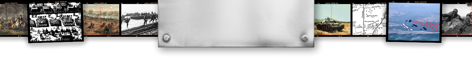
Any model of air combat needs to address the effect of weapons on the opposing forces. In the Dupuy Air Combat Model (DACM), this was rifled bullets fired from machine guns, as well as small caliber cannon in the 20-30 millimeter (mm) class. Such was the state of air combat in World War II. This page is an excellent, in-depth analysis of the fighter guns and cannon. Of course, technology has effects beyond firepower. One of the most notable technologies to go into active use during World War II was radar, contributing to the effectiveness of the Royal Air Force (RAF), successfully holding off the Wehrmacht’s Luftwaffe in the Battle of Britain.
Since that time, driven by “great power competition”, technology continues to advance the art of warfare in the air. This happened in several notable stages during the Cold War, and was on display in subsequent contemporary conflicts when client or proxy states fought on behalf of the great powers. Examples include well-known conflicts, such as the Korean and Vietnam conflicts, but also the conflicts between the Arabs and Israelis. In the Korean War, archives now illustrate than Russian pilots secretly flew alongside North Korean and Chinese pilots against the allied forces.
Stages in technology are often characterized by generation. Many of the features that are associated with the generations are driven by the Cold War arms race, and the back and forth development cycles and innovation cycles by the aircraft designers. This was evident in comments by Aviation Week’s Bill Sweetman, remarking that the Jas-39 Grippen is actually a sixth generation fighter, based upon the alternative focus on maintainability, operability from short runways / austere airbases (or roadways!), the focus on cost reduction, but most importantly, software: “The reason that the JAS 39E may earn a Gen 6 tag is that it has been designed with these issues in mind. Software comes first: The new hardware runs Mission System 21 software, the latest roughly biennial release in the series that started with the JAS 39A/B.”
Upon close inspection of the DACM parameters, we can observe a few important data elements and metadata definitions: avionics (aka software & hardware), and sensor performance. Those two are about data and information. A concise method to assign values to these parameters is needed. The U.S. Air Force (USAF) Air Combat Command (ACC) has used the generation of fighters as a proxy for this in the past, at least at a notional level:
[Source: 5th Generation Fighters, Lt Gen Hawk Carlisle, USAF ACC]
The Fleet Series game that has been reviewed in previous posts has a different method. The Air-to-Air Combat Resolution Table does not seem to resonate well, as the damage effects are imposed against either one side or the other. This does not jive with the stated concerns of the USAF, which has been worried about an exchange in which both Red and Blue forces are destroyed or eliminated in a mutual fashion, with a more or less one-for-one exchange ratio.
The Beyond Visual Range (BVR) version, named Long Range Air-to-Air (LRAA) combat in Asian Fleet, is a better model of this, in which each side rolls a die to determine the effect of long range missiles, and each side may take losses on non-stealthy units, as the stealthy units are immune to damage at BVR.
One important factor that the Fleet Series combat process does resolve is a solid determination of which side “holds” the airspace, and this is capable of using other support aircraft, such as AWACS, tankers, reconnaissance, etc. Part of this determination is the relative morale of the opposing forces. These effects have been clearly evident in air campaigns such as the strategic bombing campaign on Germany and Japan in the latter portion of World War II.
Dealing with this conundrum, I decided to relax by watching some dogfight videos on YouTube, Dogfights Greatest Air Battles, and this was rather entertaining, it included a series of engagements in aerial combat, taken from the exploits of American aces over the course of major wars:
Eddie Rickenbacker, flying a Spad 13 in World War I,
Clarence Emil “Bud” Anderson, flying a P-51B “Old Crow” in European skies during World War II, flying 67 missions in P-51Ds, 35 missions in F-80s and 121 missions in F-86s. He wrote “No Guts, No Glory,” a how to manual with lots of graphics of named maneuvers like the “Scissors.”
An interesting paraphrase by Cunningham of Manfred von Richthofen, the Red Baron’s statement: “When he sees the enemy, he attacks and kills, everything else is rubbish.” What Richthofen said (according to skygod.com), was “The duty of the fighter pilot is to patrol his area of the sky, and shoot down any enemy fighters in that area. Anything else is rubbish.” Richtofen would not let members of his Staffel strafe troops in the trenches.
The list above is a great reference, and it got me to consider an alternative form of generation, including the earlier wars, and the experiences gained in those wars. Indeed, we can press on in time to include the combat performance of the US and Allied militaries in the first Gulf War, 1990, as previously discussed.
There was a reference to the principles of aerial combat, such as the Dicta Boelcke:
Secure the benefits of aerial combat (speed, altitude, numerical superiority, position) before attacking. Always attack from the sun.
If you start the attack, bring it to an end.
Fire the machine gun up close and only if you are sure to target your opponent.
Do not lose sight of the enemy.
In any form of attack, an approach to the opponent from behind is required.
If the enemy attacks you in a dive, do not try to dodge the attack, but turn to the attacker.
If you are above the enemy lines, always keep your own retreat in mind.
For squadrons: In principle attack only in groups of four to six. If the fight breaks up in noisy single battles, make sure that not many comrades pounce on an opponent.
Appendix A – my own attempt to classify the generations of jet aircraft, in an attempt to rationalize the numerous schemes … until I decided that it was a fool’s errand:
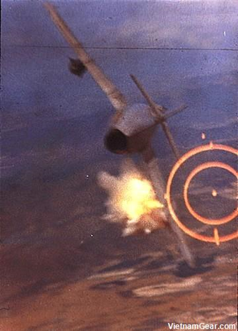
Jeffrey H Michaels, a Senior Lecturer in Defence Studies at the British the Joint Services Command and Staff College, has published a detailed look at how Hackett and several senior NATO and diplomatic colleagues constructed the scenario portrayed in the book. Scenario construction is an important aspect of institutional war gaming. A war game will only be as useful if the assumptions that underpin it are valid. As Michaels points out,
Regrettably, far too many scenarios and models, whether developed by military organizations, political scientists, or fiction writers, tend to focus their attention on the battlefield and the clash of armies, navies, air forces, and especially their weapons systems. By contrast, the broader context of the war – the reasons why hostilities erupted, the political and military objectives, the limits placed on military action, and so on – are given much less serious attention, often because they are viewed by the script-writers as a distraction from the main activity that occurs on the battlefield.
Modelers and war gamers always need to keep in mind the fundamental importance of context in designing their simulations.
It is quite easy to project how one weapon system might fare against another, but taken out of a broader strategic context, such a projection is practically meaningless (apart from its marketing value), or worse, misleading. In this sense, even if less entertaining or exciting, the degree of realism of the political aspects of the scenario, particularly policymakers’ rationality and cost-benefit calculus, and the key decisions that are taken about going to war, the objectives being sought, the limits placed on military action, and the willingness to incur the risks of escalation, should receive more critical attention than the purely battlefield dimensions of the future conflict.
These are crucially important points to consider when deciding how to asses the outcomes of hypothetical scenarios.
This is like saying, “A team can’t score in football unless it has the ball.” Although subsequent verities stress the strength, value, and importance of defense, this should not obscure the essentiality of offensive action to ultimate combat success. Even in instances where a defensive strategy might conceivably assure a favorable war outcome—as was the case of the British against Napoleon, and as the Confederacy attempted in the American Civil War—selective employment of offensive tactics and operations is required if the strategic defender is to have any chance of final victory. [pp. 1-2]
Only offensive action achieves decisive results. Offensive action permits the commander to exploit the initiative and impose his will on the enemy. The defensive may be forced on the commander, but it should be deliberately adopted only as a temporary expedient while awaiting an opportunity for offensive action or for the purpose of economizing forces on a front where a decision is not sought. Even on the defensive the commander seeks every opportunity to seize the initiative and achieve decisive results by offensive action. [Original emphasis]
Interestingly enough, the offensive no longer retains its primary place in current Army doctrinal thought. The Army consigned its list of the principles of war to an appendix in the 2008 edition of FM 3-0 Operations and omitted them entirely from the 2017 revision. As the current edition of FM 3-0 Operations lays it out, the offensive is now placed on the same par as the defensive and stability operations:
Unified land operations are simultaneous offensive, defensive, and stability or defense support of civil authorities’ tasks to seize, retain, and exploit the initiative to shape the operational environment, prevent conflict, consolidate gains, and win our Nation’s wars as part of unified action (ADRP 3-0)…
At the heart of the Army’s operational concept is decisive action. Decisive action is the continuous, simultaneous combinations of offensive, defensive, and stability or defense support of civil authorities tasks (ADRP 3-0). During large-scale combat operations, commanders describe the combinations of offensive, defensive, and stability tasks in the concept of operations. As a single, unifying idea, decisive action provides direction for an entire operation. [p. I-16; original emphasis]
It is perhaps too easy to read too much into this change in emphasis. On the very next page, FM 3-0 describes offensive “tasks” thusly:
Offensive tasks are conducted to defeat and destroy enemy forces and seize terrain, resources, and population centers. Offensive tasks impose the commander’s will on the enemy. The offense is the most direct and sure means of seizing and exploiting the initiative to gain physical and cognitive advantages over an enemy. In the offense, the decisive operation is a sudden, shattering action that capitalizes on speed, surprise, and shock effect to achieve the operation’s purpose. If that operation does not destroy or defeat the enemy, operations continue until enemy forces disintegrate or retreat so they no longer pose a threat. Executing offensive tasks compels an enemy to react, creating or revealing additional weaknesses that an attacking force can exploit. [p. I-17]
The change in emphasis likely reflects recent U.S. military experience where decisive action has not yielded much in the way of decisive outcomes, as is mentioned in FM 3-0’s introduction. Joint force offensives in 2001 and 2003 “achieved rapid initial military success but no enduring political outcome, resulting in protracted counterinsurgency campaigns.” The Army now anticipates a future operating environment where joint forces can expect to “work together and with unified action partners to successfully prosecute operations short of conflict, prevail in large-scale combat operations, and consolidate gains to win enduring strategic outcomes” that are not necessarily predicated on offensive action alone. We may have to wait for the next edition of FM 3-0 to see if the Army has drawn valid conclusions from the recent past or not.
It is my understanding that he was the person who was responsible for making sure that DACM (Dupuy Air Combat Model) was funded by AFSC. He then retired from the Air Force in 1994. We completed the demonstration phase of the DACM and quite simply, there was no one left in the Air Force who was interested in funding it. So, work stopped. I never met General McInerney and was not involved in the marketing of the initial effort.
But, this is typical of the problems with doing business with the Pentagon, where an officer will take an interest in your work, generate funding for it, but by the time the first steps are completed, that officer has moved on to another assignment. This has happened to us with other projects. One of these efforts was a joint research project that was done by TDI and former Army surgeon on casualty rates. It was for J-4 of the Joint Staff. The project officer there was extremely interested and involved in the work, but then moved to another assignment. By the time we got original effort completed, the division was headed by an Air Force Colonel who appeared to be only interested in things that flew. Therefore, the project died (except that parts of it were used for Chapter 15: Casualties, pages 193-198, in War by Numbers).
Our experience in dealing with the U.S. defense establishment is that sometimes research efforts that takes longer than a few months will die……because the people interested in it have moved on. This sometimes leads to simple, short-term analysis and fewer properly funded long-term projects.
Last night, as I was watching the Capitals trash Tampa Bay in the third round of the Stanley Cup play-offs….the announcer mentioned that only twice in the last 41 years (or cases) has a team won the third round of the play-offs after loosing the first two games. Tampa Bay was lost the first two games. So, historically, in only 4.878% (say 5%) of the cases has someone come back from loosing the first two play-off games to win. Note that the Capitals did this against Columbus in the first round.
Now, there are seven games in a play-off round. So with five games left, Tampa Bay has to win 4 of the 5 games. So, assuming the teams are equal (50% chance of either winning a game), then the odds of Tampa Bay winning 4 of the next 5 games I calculate as .09375 (mathematicians…please check me on this) or 9%. So if the teams are equal, then Tampa Bay should statistically have a 9% chance of coming back and winning the round. Historically, it has only happened 5% of the time.
Suppose Tampa Bay is the better team. Lets say their odds of winning are 60% for each game, then their odds of winning 4 out of 5 rises to 18.144%. They did win 2 out of 3 games against the Capitals in the regular season, so maybe their odds of winning any single game is really 67%. This is a 26.34% chance of coming back. Let us say they are really good and motivated and have a 75% of winning each game, then the odds are 39.55%. On the other hand, to get to the historical 5% win rate in this situation, then team that is behind had to have around a 42% chance of winning each game.