Category Modeling, Simulation & Wargaming

Two proposals on Combat Casualties

In my last post I referenced two proposals I prepared for the CCCRP (Combat Casualty Care Research Program) on combat casualties. This was built off Chapter 15 “Casualties” in my book War by Numbers and some combat casualty modeling work I had done at the Marine Corps Warfighting Lab (MCWL). The working level of CCCRP was very supportive of this effort, but their proposal process went through a group of reviewers, and in each case, one reviewer saw no reason to do this work. As I think the reviewers were medical doctors, and the proposals were not directly related to casualty care, it is not surprising that a couple of them would feel that way. It obviously did not fit any of their immediate needs or concerns. So, this effort died in the fall of 2020.

The two proposals were:

  1. Combat Analysis Proposal of three tasks:
    1. Ratios for operations: A brief exploration of existing sources to determine what the expected wounded-to-killed ratios are for different types of operations. This would include a projection for 1) modern (post-World War II) conventional combat scenarios, 2) modern counter-insurgencies, 3) modern training and assistance missions, and 4) special operations and other active assistance programs. The goal would be to assemble a set of figures that can then be applied to combat model outputs, planning, and other studies and analysis.
    2. Ratios by Posture: Conduct a detailed analysis of division-level conventional combat to determine the wounded-to-killed ratios dependent on outcome and posture. This will be a comparative analysis based upon the coded outcomes of the engagements in the database and whether the force is conducting an offensive, defensive or other type of mission. The goal is to determine if wounded-to-kill ratios vary in these conditions (which they certainly do) and to determine to what extent they do and what are those values.
    3. Lethality of IEDs: Develop a set of values for the lethality of modern IEDs (Improvised Explosive Devices), booby traps, mines, claymores, truck bombs, suicide bombers, and other such devices. The lethality figures will have to be developed from a systematic review of a variety of combat and medical reports. Ideally, this data can be assembled from the experiences in Iraq and Afghanistan, but research will also examine various operations in the Middle East, Northern Ireland, Vietnam and other post-WWII insurgencies. This would also include a review of the Wound Data and Munitions Effectiveness Team (WDMET) data from the Vietnam War and the ongoing Joint Theater Trauma Registry (JTTR).
  2. Combat Modeling Proposal of three tasks:
    1. Lethality Rates: A brief exploration of existing sources to determine what the lethality rates are for various weapons. This effort will tap existing open sources and is an extension of the work outlined in Chapter 15, “Casualties” in the book War by Numbers.
    2. How Models Measure Casualties: Conduct a review of around a half-dozen active U.S. Army and DOD conventional combat models and determine how they measure casualties and how they determine wounded versus killed (and missing). This review will probably include meetings with the modelers, in additional to conducting an analysis for the differences between their various approaches.
    3. Medical Deployment Options for Conventional Operations: Conduct a comparative simulation of medical care, evacuation and return-to-duties over an extended conventional warfare exercise. This would be an examination of the optimal medical support structure of the sake of sustaining combat power over an extended conventional deployment.
      1. The three recommended scenarios are 1) Emergency deployment to the Baltic States, 2) intervention in collapsed state of North Korea, and 3) the validation scenario for Iraq in 2006. Other scenarios may be added time permitting, or as a possible future effort.

This was the last time I attempted to market DOD. It took some man-months of effort to assemble and submit these proposals along with all the required supporting documentation. There is a trade-off of whether my time is better spent looking for the next contract or writing my next book. I decided after this experience to focus on writing my next books, which is why I now have two completed books going through editing and am about to contract for two more books. It is difficult for a small company to work for the DOD. The number of hoops and time consumed in marketing efforts are the same whether it is Lockheed Martin or TDI. Anyhow, if CCCRP would not approve such an effort, then I do not know who in DOD would. As it is, I gave up trying to further market it and prioritized my time to other projects.

A Second Independent Effort to use the QJM/TNDM to Analyze the War in Ukraine

This is the second such effort we are presenting. The first is here: An Independent Effort to Use the QJM to Analyze the War in Ukraine | Mystics & Statistics (dupuyinstitute.org)

We have had no involvement in either effort, although we have had a relationship with the author of this second effort that dates back to the early 1990s. The research, results, analysis and conclusions are entirely the author’s own. TDI has had no involvement in preparing this.

This second analysis is done by William (Chip) Sayers, the author of this posting: A story about planning for Desert Storm (1991) | Mystics & Statistics (dupuyinstitute.org). He will be doing a presentation at the HAAC: Schedule of the Historical Analysis Annual Conference (HAAC), 27-29 September 2022 – update 6 | Mystics & Statistics (dupuyinstitute.org)

The version of the model Chip Sayers used was an earlier “pre-programmed” version of the TNDM. Do not know exactly what all is included in it or not included. He assisted Trevor Dupuy in revising the formula for the OLI’s as it addressed modern armor. It was part of a master thesis he was working on.

Anyhow, his presentation is below:


————————–prepared by William Sayers—————————

Since the 26th of February (two days after Russia invaded Ukraine), two questions have been begging to be answered: 

  1. How have the Ukrainians managed to thwart the Russian Army?
  2. Was Ukrainian success foreseeable?

In order to explore these questions, I set up a hypothetical battle from the first few days of the war and analyzed it using The Dupuy Institute’s Tactical Numerical Deterministic Model (TNDM).  My first task was to see if the TNDM is capable of recreating battlefield results similar to what we are seeing in Ukraine.  If the TNDM could approximate the losses and movement of forces that we are seeing come out of this war, it would validate the utility of the model. 

Having determined that the model is relevant, I could move on to my second objective, which was to determine if the performance of the Ukrainian and Russian Armies was something that should have been foreseeable or was an edge case that couldn’t have been predicted.  My format was to run a base case with no quality modifier to either side, and then two more where the Ukrainian side was given a Combat Effectiveness Value (CEV) of 1.2 for the second run, and 1.5 for the third.  I believe there is every reason to give the Ukrainians a CEV advantage; the only question is to what magnitude.

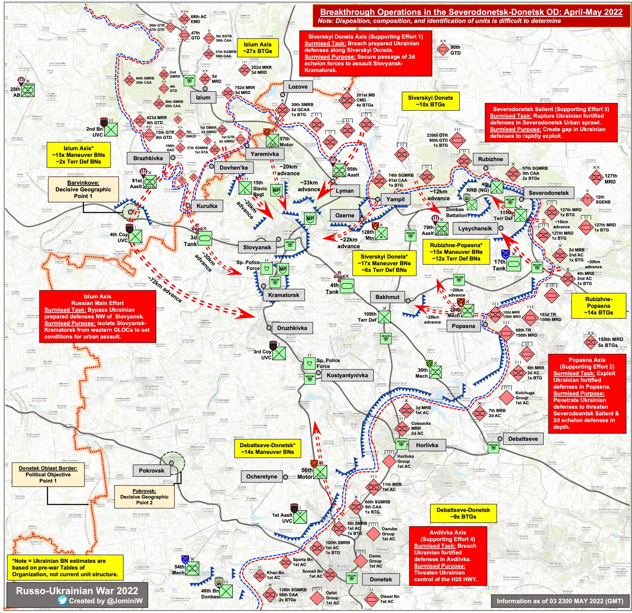
I began by putting together an Order of Battle for the two sides using various sources available openly on the web.  While the units involved are (I believe) real and constituted roughly as I have presented them, the units pitted against one another, their operations and missions are meant to be representative and not necessarily a depiction of actual operations.

Initial observations:

  • Russian doctrine allows for the possibility of a successful operation at the Front-level with a Correlation of Forces (measuring combat potential in both quantitative and qualitative terms) superiority of as little as 1.2:1. Comparing the forces in this case, the Russian Ground Order of Battle : Ukrainian Ground Order of Battle = 1.5:1.  However, If terrain is added (rolling, gentile, mixed = 1.3) to a Ukrainian posture of 1.3 (hasty defense), the CoF is driven below unity.  As the Russian troops have proven to be poorly trained and unmotivated conscripts and the Ukrainians are fighting in their homeland against a very brutal aggressor, a Combat Effectiveness Value (troop quality) advantage seems to be called for and would serve to drive the overall CoF even further in Ukraine’s favor.  Conclusion: The Russian General Staff clearly erred in believing that they had sufficient force to fight this war.  They seem to have gambled on a political collapse on Kiev’s part, and when that did not happen, they were stuck in a losing battle.
  • Early claims that the Russian Army had committed 85% of its combat strength to the operation appear to be justified. Every military district has contributed major forces, including the Eastern Military District adjoining the Pacific Ocean.  The upshot is that if the Russian Army does not win this war politically, or on the battlefield with the forces on hand, there is very little hope that they can reinforce sufficiently to win with what they can use of the other 15% of the Russian Army.

Wargame Narrative:

Concept of Operations: Russian 35th and 36th Combined Arms Armies attack in the vicinity of the tri-border area with river crossing of Pripyat River:  the 35th CAA attack with the 38th Guards and 64th Independent Motorized Rifle Brigades at Pripyat, with the 35th in the lead and the 64th in the second echelon and supported by the 165th Artillery Brigade, 30 x Mi-24 and 20 x Su-25 sorties, and the 69th Independent Covering Brigade in reserve.  The 36th CAA attacks at the city of Chernobyl with the 5th and 37th Guards Tank Brigades supported by the 200th Artillery Bde, 30 x Mi-24 and 20 x Su-25 sorties.  The 29th Combined Arms Army constitutes the Front’s 2nd echelon.

The Ukrainian 14th Mechanized Brigade plus ½ of the 38th Artillery Brigade and 20 x Mi-24 sorties defends vs. 35th CAA, while the Ukrainian 15th Mech Bde plus ½ of the 38th Arty Bde, 20 x Mi-24 sorties defends vs. 36th CAA.

Day 1:

The Ukrainian 14th Mechanized Brigade rebuffs the 38th Guards Independent Motorized-Rifle Brigade, which takes heavy losses and fails to cross the river opposite the defunct nuclear power plant.  The 38th Brigade loses 17% of its combat power, four aircraft, nearly half its armored vehicles and 215 KIA, seriously wounded and captured.

On the southern axis, the 5th Guards Tank Brigade crosses the Pripyat River and secures the highway bridge north of town.  The 37th Guards Tank Brigade successfully crosses directly into Chernobyl City and both brigades push 1 ¼ km beyond the river.  Losses include 176 troops, 27 AFVs and 2 aircraft.

Day 2:

The 14th Mech Brigade frustrates a second attempt to force a river crossing.  The 38th Bde loses another 4 aircraft and 24 armored vehicles, bringing their total losses to over 80% of their tanks and infantry fighting vehicles.  Personnel losses now total over 420 men.

In the south, the 5th and 37th Guards Tank Brigades continue to push through the town of Chernobyl, making another 1.5km at minimal loss.

Day 3:

Having lost 30% of their combat power after two days of unsuccessful river crossing ops, the 38th Guards Ind. MR Bde has been temporarily rendered combat ineffective.  They drop into a holding posture and attempt to fix in place the 14th Mech while minimizing further casualties.  Rather than attempt passing the second echelon through, the 64th Guards wait in readiness for the 36th CAA to flank 14th Mech and make their position untenable.  Total losses stand at 60 out of 71 tanks and IFVs, 8 aircraft and 475 troops.

The 36th CAA has pushed the 15th Bde out of its prepared positions forcing them into a hasty defense posture and accelerating their advance rate to 2km per day.  This opens up a gap between the Ukrainian 14th and 15th Mech Bdes, threatening their supporting 38th Artillery Brigade.  The 38th is forced to displace to the south, behind the 15th Mech.  Meanwhile, the 14th Mech’s right flank is now fully exposed.  Russian losses after three days on the 36th CAA’s axis are 75 tanks and IFVs, 6 aircraft and 483 men.

Observations after 3 days:

  • The only viable river crossing area in the vicinity of the Chernobyl nuclear facility was the area around the railroad bridge. This was a tight squeeze for a single brigade with swampy ground to either side.  This left the Russians to attack the defending Ukrainian brigade at a CoF ratio of less than 1:1, yielding high losses and a stalled attack.  The Russians’ only hope was to fix the Ukrainian defenders in place and wait for the 36th CAA to turn north into the 14th Mech’s flank.
  • With over twice the combat power available, the 36th CAA was able to successfully make its river crossing at Chernobyl city and continuously push back the defenders. Eventually this opened up the opportunity to wedge the 14th Mech out of their positions near the reactor complex.
  • In just three days the Russians lost nearly 1,000 men (of which, ~250 would have been KIA), 135 tanks and IFVs and 14 fixed-wing aircraft and helicopters. If this exercise represents one of eight major axes of advance with similar combat intensities, even the higher published estimates of Russian losses seem plausible.
  • In contrast, Ukrainian losses were somewhat lower: 61 tanks and IFVs, 16 helicopters and 794 men (of which ~200 would have been KIA).
  • The highest rate of advance the Russians achieved was 2km per day, considerably slower than their Cold War expectations. Beginning on day 4, the Ukrainians would have had to reposition lest the 14th Brigade be isolated and destroyed.  Once the defenders broke contact, Russian advance rates would have picked up considerably.  At that point, it would be a game of hit and run by the defenders, trading space for casualties until they found another favorable terrain feature with which to anchor their line.  Clearly, the Ukrainians proved capable of mounting a serious defense against the invading force, both in the model and on the ground.

The battle was replayed twice to explore the impact of a Ukrainian advantage in Combat Effectiveness Value, once with a 20% advantage, and once with a 50% superiority.  As mentioned earlier, a CEV superiority for the Ukraine can be assumed because Russian conscripts have proven to be poorly trained and unmotivated while the Ukrainians are fighting in their homeland against a very brutal and existential threat.  These runs were made with the intent of finding the extent of that CEV superiority.

Ukrainian CEV of 1.2

Day 1:

The 38th Guards Ind. MR Bde takes heavy losses, fails to cross river opposite the defunct nuclear power plant.  38th Bde loses 26% of its combat power, five aircraft, over ¾’s its armored vehicles and 283 KIA, seriously wounded and captured.

The 5th Guards Tank Brigade crosses the Pripyat River and secures the highway bridge north of town.  The 37th Guards Tank Brigade successfully crosses directly into Chernobyl City and both brigades push 1 km beyond the river.  Losses include 226 troops, 42 Armored Fighting Vehicles and 3 aircraft.

Day 2:

The Ukrainian 14th Mech Brigade frustrates a second attempt to force a river crossing.  The 38th Bde loses another 6 aircraft and the rest of its armored vehicles.  Personnel losses now total over 550 men.  Having lost nearly 50% of its combat power, the 38th Bde is now combat ineffective.

The 5th and 37th Guards Tank Brigades continue to push through the town of Chernobyl, making another 1.2km, losing 39 tanks and IFVs, 3 aircraft and 211 men.

Day 3:

The 36th CAA continues to slowly push the 15th Bde at a rate of 1.3km per day at a total cost of 9 aircraft, 117 AFVs and 636 men, with a total advance of 3.5 km in three days.

Observations:  The battle developed in much the same way as the base run (no CEV advantage), but more slowly and at higher cost to the Russians. 

Ukrainian CEV of 1.5

Day 1:

The 38th Guards Ind. MR Bde takes heavy losses, fails to cross river opposite the defunct nuclear power plant.  38th Bde loses eight aircraft, all of its armored vehicles and 400 men KIA, seriously wounded and captured. Having lost 64% of its combat power, the 38th Bde is rendered combat ineffective on day 1 of the operation.

The 5th Guards Tank Brigade crosses the Pripyat River and secures the highway bridge north of town.  The 37th Guards Tank Brigade successfully crosses directly into Chernobyl City and both brigades push 500m beyond the river.  Losses include 301 troops, 70 AFVs and 3 aircraft.

Day 2:

The 5th and 37th Guards Tank Brigades continue to push through the town of Chernobyl, making another 600m, losing 74 tanks and IFVs, 4 aircraft and 287 men.

Day 3:

The 36th CAA continues to slowly push the 15th Bde at a rate of 700m per day at a total cost of 11 aircraft, 201 AFVs and 840 men. 

Observations:

The Russian force trying to cross the river at the power plant ran into a brick wall.  The rest of the operation continued to develop along the lines of the base case, but at a snail’s pace.  It was not entirely certain that the operation would continue before losses brought it to a halt.  Given that Russian troops took control of the power plant fairly rapidly, a 1.5 CEV is probably too large an advantage.  The 1.2 CEV case fits the results better.

Outlook:

  • Given their failure to cause a collapse of political will by indiscriminate bombing and shelling of Ukrainian cities and the probable combat attrition of Russian forces, the redeployment of the Russian Army to the Donbas region seems more of an attempt to salvage something from this campaign gone wrong, rather than a war-winning strategy. Ukrainian forces can redeploy more easily and have likely suffered a smaller percentage of losses than the Russian Army and thus should be in a relatively better position according to the Correlation of Forces than they were at the beginning of the invasion.  Given an upwards of 85% of the Russian Army was committed to the operation, it is highly doubtful that they have significant forces to send as reinforcements.  For instance, it is essentially impossible for Russia to deploy the 11th Army Corps from Kaliningrad to Ukraine as reinforcements, yet they make up as much of 30% of the combat power of the Russian Army not yet committed to Ukraine.
  • The lack of accurate OOB and combat loss information make it impossible to make a confident prediction on the future course of the war. However, one can be fairly confident that the Russians will not be able to mount successful major offensive operations – they are played out and only the massive use of chemical weapons, or the use of tactical nuclear weapons is likely to change the course of the war.  They apparently intend to make a play for Odessa, but it is doubtful that they will be able to successfully cross the major rivers between their forces and the objective, much less sustain operations beyond them.
  • The Ukrainian Army has made successful local counterattacks and could possibly mass sufficient combat power to push the Russian Army back to their pre-24 February positions, and possibly out of Ukraine altogether. However, it is more likely that both sides will lose – Russia will not get the territory or control Putin wants, while Ukraine will have to settle for more of their territory being occupied by Russia – at least until Putin is ousted and the UN or EU can work out a withdrawal.

What this analysis reveals about Russian Forces:  In the 1990s, Russia began a movement towards replacing the division with the brigade its main tactical grouping.  This paralleled the US Army’s development of the Brigade Combat Team to allow for greater strategic mobility.  This worked for the US, because with the massive support that could be devoted to a deployed BCT, no formation in the world the Army envisioned fighting could match the BCT’s combat power.  For the Russian Army, it appears to have been a purely economic move, with formations at most levels shrinking one echelon down (i.e., divisions became brigades, regiments became battalions, etc.)  This allowed the Russians to keep the core of the Army, while retaining a more fiscally sustainable organization.

In the 2000s to 2010s, the Russian Army experimented with going a step further, using its brigade formations to generate a Battalion Tactical Group, a reinforced, combined-arms battalion.  This seems reminiscent of British Army system of the 19th century where a regimental organization at home would deploy a battalion-sized force for expeditionary work.  The BTG system makes sense within that kind of framework, but having a brigade deploy a single battalion for a major war is untenable.  Particularly in an army whose bread and butter are mass and concentration of force.  The General Staff may have realized their mistake as they are rebuilding several divisions and may be headed for a more traditional force structure.  For this war, however, they’ve been caught with one boot on and one off.

Up to a certain point, the Russian’s traditional use of massive amounts of artillery could make up for the lack of maneuver forces.  Certainly, if the General Staff believed that rolling up to the outskirts of a city, using the maneuver forces to provide security for the guns, while the artillery batters the civilian infrastructure until the enemy’s political leadership cries uncle is a theoretically viable strategy.  But what happens if the enemy leadership doesn’t lose its nerve?  How does this pittance of scattered battalions execute a plan B to subdue the enemy?

By my estimation, the Russian Army has deployed about 21 maneuver brigades for the war in Ukraine.  Additionally, up to 42 more maneuver regiments subordinated to divisions may have been deployed.  This, against a Ukrainian force of 39 maneuver brigades.  On average, Ukrainian brigades appear to be somewhat more powerful than Russian brigades.  In an experimental run made earlier, a good Ukrainian brigade with surprise and a CEV advantage routed a weak, and unsupported Russian division.  While this run gave very favorable conditions to the Ukrainian side, there is no doubt that a Ukrainian maneuver brigade can be a formidable force.  39 of these brigades defending against 64 Russian formations of basically the same echelon may acquit itself fairly well, especially if a reasonable CEV is added to the mix.  It does not bode particularly well if the Ukrainian force must go over to the offensive.  However, if each Russian brigade is actually fielding just one reinforced battalion, the equation changes considerably.  That’s only 21 BTGs.  If the divisional regiments are organized the same way, the Russians have invaded Ukraine with 63 Battalion Tactical Groups facing the equivalent of roughly 120 battalions.  According to Clausewitz, that should be a no go by anyone’s mathematics.  

Bottom line:  I’m extremely suspicious of the idea of Battalion Tactical Groups.  Either we are not understanding them properly, or the Russians are using the term as disinformation.  I have a difficult time believing that they invaded Ukraine with 63 independent and uncoordinated battalions and had any success at all.  Worse, once the offensive was checked, the Ukrainians should have been able to make quick work of mopping up these isolated units.  If the Russians were far better at C3, there might be some viability in the BTG concept.  However, the Russians have never been known for their sophisticated Command & Control and certainly have not proven particularly good at it in the present conflict.

What this analysis reveals about Ukrainian Forces:

Initially, most pundits predicted that Ukrainian Forces would fold rapidly in the face of overwhelming Russian numerical superiority.  The TNDM analysis demonstrates that if the Ukrainians were willing to fight back with reasonable competence and vigor, they were capable of stalemating the Russian invaders short of their ultimate objectives.

After the initial shock of Ukrainian success, many analysts turned around their judgments completely and praised the Ukrainian Forces as some kind of elite David taking on a ponderous Goliath.  The TNDM shows that the success of the Ukrainian Army is not necessarily due to unusually proficient or heroic performance, but rather the expected performance of a competent force.  Given the demonstrated poor performance of Russian conscript troops, their terrible morale, and the shambles of the Russian C3 and logistics systems, one might be surprised if the Ukrainian Army didn’t perform this well.  After all, in contrast to the Russian Army, the Ukrainian’s have their backs against the wall in an existential war.  They should be performing at a higher level than Russian conscripts.  If anything, the Ukrainian Army may be underperforming.  That would bear exploration.

Implications for TDI:

The TNDM yields results that are entirely consistent with what we are seeing in the war, so far.  No other model that I have worked with comes close to this performance.  Further, it is extremely easy to use and very agile in its ability to analyze permutations, branches and sequels, and the unforeseen “what-ifs” that come up during the course of a modeling exercise.  While no substitution excursions were explored in this experiment, the model is set up well to replace one equipment set with another and measure the impact of different weapons systems and capabilities on unit performance.

The ability for the TNDM to model a campaign as it happens is limited only by the quality of the intelligence information provided.

—————————————–

Dupuy used for Click Bait

This was also just sent to me: The Deadliest Weapon of all Time.

They are using a 1964 report by Trevor Dupuy to create one those little click bait articles. The original report (#4) is here: TDI – The Dupuy Institute Publications

Number 16: That does not look like a medieval crossbow. I would know. I have one hanging over my fireplace.

Number 8: Pretty certain that picture is not of a World War I fighter-bomber. While they did use monoplanes in the Great War (1914-1918), few had fully enclosed cockpits.

Anyhow, entertained. Works as click bait.

Also see: Two ARL Reports | Mystics & Statistics (dupuyinstitute.org) and Technological Advancement Lessons from History? | Mystics & Statistics (dupuyinstitute.org). Dr. Kott is schedule to speak at our conference in September:  Schedule of the Historical Analysis Annual Conference (HAAC), 27-29 September 2022 – update 6 | Mystics & Statistics (dupuyinstitute.org).

Talking Force Ratios Once Again

I guess we need to talk about force ratios once again. Not sure why. This has been discussed in depth by us. It was discussed in Trevor Dupuy’s Understanding War and was discussed in my book War by Numbers. But let me start first with some Clausewitz quotes:

In tactics, as in strategy, superiority of numbers is the most common element in victory.

and

If we thus strip the engagement of all the variables arising from its purpose and circumstance, and disregard the fighting value of the troops involved (which is a given quantity), we are left with the bare concept of the engagement, a shapeless battle in which the only distinguishing factors is the number of troops on either side.

These numbers, therefore, will determine victory. It is, of course, evident from the mass of abstractions I have made to reach this point that superiority of numbers in a given engagement is only one of the factors that determines victory. Superior numbers, far from contributing everything, or even a substantial part, to victory, may actually be contributing very little, depending on the circumstances.

But superiority varies in degree. It can be two to one, or three or four to one, and so on; it can obviously reach the point where it is overwhelming.

In this sense superiority of numbers admittedly is the most important factor in the outcome of an engagement, as long as it is great enough to counterbalance all other contributing circumstance. It thus follows that as many troops as possible should be brought into the engagement at the decisive point.

and also:

Numerical superiority was a material factor. It was chosen from all elements that make up victory because, by using combinations of time and space, it could be fitted into a mathematical system of laws. It was thought that all other factors could be ignored if they were assumed to be equal on both sides and thus cancelled one another out. That might have been acceptable as a temporary device for the study of the characteristics of this single factor; but to make the device permanent, to accept superiority of numbers as the one and only rule, and to reduce the whole secret of the art of war to a formula of numerical superiority at a certain time and a certain place was an oversimplification that would not have stood up for a moment against the realities of life.

OK…in its most basic form, combat power is numbers x equipment x human factors x conditions of combat (including posture, terrain, weather, surprise, etc.). Nothing earthshaking here, but this often gets lost in the discussion. 

In Trevor Dupuy’s Understanding War, which is his most significant work, he has Chapter 3: Clausewitz’s Theory of Combat, which has a section on “The Law of Numbers.” and Chapter 4: “The Three-to-one Theory of Combat.” These are worth reading.

My book War by Numbers covered some of the same ground. Chapter Two is called “Force Ratios.”

An article from the Wall Street Journal was published on Friday that addressed this subject, somewhat incompletely: https://www.wsj.com/articles/how-a-simple-ratio-came-to-influence-military-strategy-11652434202. The author did reach out to me by email on 27 April, but I don’t check that mail box that often, so never got back to him in time for the article.

I am not going to discuss or debate this article, but instead point out that this has been discussed before. So not sure why we are back drinking from the same well using the same tables that we know are not correct. In particular I am talking about the table from the U.S. Army’s COFM (Correlation of Forces and Means).

This is discussed in this blog post: How Does the U.S. Army Calculate Combat Power? ¯\_(ツ)_/¯ | Mystics & Statistics (dupuyinstitute.org)

Table in question is here:

A copy of the COFM is here: COFM. Do not know if this is the most current or recent version, nor do I care, because it is flawed.

We have discussed this many times before. See: How Does the U.S. Army Calculate Combat Power? ¯\_(ツ)_/¯ | Mystics & Statistics (dupuyinstitute.org) and TDI Friday Read: The Validity Of The 3-1 Rule Of Combat | Mystics & Statistics (dupuyinstitute.org) and Summation of Human Factors and Force Ratio posts | Mystics & Statistics (dupuyinstitute.org) and Summation of Force Ratio Posts | Mystics & Statistics (dupuyinstitute.org).

The COFM is called out five times in the ATP 5-0.2-1 Staff Reference Guide. The guide is discussed here: Staff Reference Guide | Mystics & Statistics (dupuyinstitute.org).

Other people have also discussed this:  

1993: Correlation of Forces: The Quest for a Standardized Model by Major David Hogg: Correlation of Forces. Note that the COFM table is quote in figure 1 in this paper.

2007 or later: Demystifying the Correlation of Forces Calculator: https://www.benning.army.mil/infantry/Magazine/issues/2017/JAN-MAr/pdf/7)Spurlin_CoFCalculator_txt.pdf. They reference the paper above by LTG (then Major) David Hogg.

2019: An Examination of Force Ratios: https://apps.dtic.mil/sti/pdfs/AD1083211.pdf. This last paper actually references my book War by Numbers.

An Independent Effort to Use the QJM to Analyze the War in Ukraine

The QJM is the old version of Trevor Dupuy’s Quantified Judgment Model, as described in his book Numbers, Predictions and War. The Dupuy Institute currently uses and markets the TNDM (Tactical Numerical Deterministic Model), which is Trevor Dupuy’s updated version of the model.

We have recently had various discussions about staffing The Dupuy Institute so as to conduct analysis of various conflicts and potential conflicts around the world and publishing the results for the general public. So far, these discussions have not generated the budget to do so.

On the other hand, even though The Dupuy Institute is not doing this, we have discovered that some other people that are independently doing this. They are using the openly published versions of the QJM for their work (there were updates made to the QJM that were not published). None of this was coordinated with us and we only discovered it through twitter though the account of Jomini of the West at @JominiW

One of his more interesting tweets is that one: 

I have no idea how accurate this map is and have been hesitant to post it before.

The modeling effort being done is by @HM_Schlottman and @HelloMrBond. They summarize their effort as:

Now, it does appear that their analysis is a “paper and pencil” analysis done using that which is derived from Understanding War, vice using the entire model as described in Numbers, Predictions and War.

Just to talk through what they did:

  1. They analyzed a division-sized engagement (33,0000 vs 23,000)
  2. Terrain was given as rugged mixed/urban.
  3. Season was spring-temperate
  4. Defense was “prepared”
  5. Not sure what they did with air superiority, but it appears that they made it equal. Pretty sure that Russia still has air superiority. On the other hand, the Ukrainian intelligence assets are vastly superior (being American), and one of the aspects of air superiority is superior intelligence, so this may be a good compromise selection for now.
  6. They give Ukraine a morale advantage (basically multiplying Russia’s combat power by 0.8), but not a big one. More on this in a subsequent post, as I know someone who is doing a similar QJM based analysis.
  7. They do conclude that combat power advantage lies with the Russians at 1.4-to-1 ratio, which “is sufficient to achieve a breakthrough.”

Now, I always hate to comment on other people using the QJM. First, I am glad to see that they are using it and second, it is an estimation. My biggest fear is that my comments will turn into the “death by a thousand cuts,” masking what I think is otherwise worthwhile effort. But, I do have to make a few comments. Hopefully, they will not appear overly critical.

First, having a force preponderance does not mean a breakthrough. It means the Russians should advance. As they advance, they may achieve a breakthrough, dependent on the depth of the defender and the changing conditions of the battlefield. The model does determine win, lose or draw and rate of advance in kilometers. It does not determine whether there is a breakthrough or not. That has to be determined by the depth of the defender versus the distance advanced, often over several days. Obviously, when the distance advanced exceeds the defender’s depth, a breakthrough is achieved. This usually takes several days. As this development of the battle is often modeled using maps, acetates and grease pencils, then over the course of several days, conditions are likely to change, with the defender either being reinforced, or withdrawing, or other counterattacks or operations developing. This starts getting complex and is where the analyst takes over from the model.

Second, the force strengths for both sides “does not include supporting arms outside of BTGs (artillery, air defense, logistics brigades, etc.).” Well, the supporting material, translated into combat power in the form of supporting artillery and supporting air and drone strikes, is significant. In some battles the supporting air and artillery for an operation makes up the majority of the combat power. Not sure how you model that with any confidence in the current situation, but they do matter.

Third, he used his own combat power formula. So, for example, he made the combat power of a tank equal to “75 troops + their share of supporting weapons.” This is certainly a simplification, but probably one he had to do as researching and scoring all the weapons is a fairly time consuming process. The original QJM has a formula for calculating the combat power of each and every weapon, and then their combat power were modified by the conditions of combat. The TNDM used a revised formula for armor vehicles that we developed by Chip Sayers, the author of this blog post: A story about planning for Desert Storm (1991) | Mystics & Statistics (dupuyinstitute.org). He will be presenting at our conference in September: Schedule of the Historical Analysis Annual Conference (HAAC), 27-29 September 2022 – update 6 | Mystics & Statistics (dupuyinstitute.org).

Now, there is a wonderfully detailed chart dated 1 May 22 on the right side of their graphic that is worth looking at. You do have to copy the image and blow it up. But it is clear that it is the basis for his strength estimates. It would be nice to get a full explanation of what he is looking at here and what it says.

Anyhow, that is all on the QJM analysis so far. It is looking at a fight around Izium and I gather north of Sievierdonetsk. I gather it concludes that the Russians should be advancing. I don’t see anything here I fundamentally disagree with.

I am assuming that @JominiW, @HM_Schlottman and @HelloMrBond are following this blog. None are known to me, but they are welcome to contact me at LawrenceTDI@aol.com.

The 88th Infantry Division Stole a Cake

Speaking of war crimes, I spotted this story today: US Army ‘returns’ cake to Italian woman for 90th birthday.

The 88th Infantry Division in Italy in 1944 in one of the units we have studied in some depth. There was a report done on it in 1981. See: 88. Performance of The 88th Infantry Division in World War II: Factors Responsible for its Excellence (1981) (MRA&L) – Pages: 120 at http://www.dupuyinstitute.org/tdipub1tnda.htm

This is also discussed on pages 114-121 of Trevor Dupuys Understanding War. He ended up conducting an analysis of the CEVs (Combat Effectiveness Values) of seven U.S. units, five UK units and 12 Germans units in Italy during WWII. This was done using his Quantified Judgment Method of Analysis (QJMA). Of those 24 units, the 88th Infantry Division was rated the fifth highest, based upon 4 engagements. It had a CEV of 1.14. It was the highest rated of all the allied units.

Ordering info is here: http://www.dupuyinstitute.org/booksfs.htm

Related posts:

Human Factors In Warfare: Combat Effectiveness | Mystics & Statistics (dupuyinstitute.org)

A story about planning for Desert Storm (1991)

In an email exchange with retired DIA (Defense Intelligence Agency) analyst, William (Chip) Sayers, he sent me this account. I asked him if we could publish it, as I think it is a wonderfully unfiltered account. He agreed, although pointed out that he would also be covering some of this in his presentation this fall. It is on Day 2 of HAAC and is on “The Combat Assessment Technique.” See: Schedule for the Historical Analysis Annual Conference (HAAC), 27-29 September 2022 – update 4 | Mystics & Statistics (dupuyinstitute.org).

In early 1989, I went to work at an office at DIA that specialized at looking at the world through the eyes of the Soviet General Staff. In particular, we used the Soviet’s Correlation of Forces Methodology. However, we only partially understood it and needed some data to close gaps for us. I cast around for something that would plug these holes and settled on the QJM as the best candidate. It was my belief that both models had approached the subject from the same standpoint and therefore the one could help inform the other.

This paid off — to an extent — in the run up to the ground campaign of Operation DESERT STORM. Gen. Schwarzkopf desperately wanted to know at what point he should let loose his ground forces and so had his staff casting about for a methodology that would give him a way to measure the success of the air campaign in softening up the Iraqis. You would think that after the years we put into WEI/WUVs and all the various models that J-8 and others used, we would have had a good basis for solving his problem. Well, you’d be wrong. Very wrong. As an illustration, Schwarzkopf claimed after the war that, in the summer of 1990, CENTCOM had gamed out the exact scenario that actually occurred and got the exact same results. Schwarzkopf was channeling his inner Nimitz, but I guarantee you that was impossible. I spent several years in the bowels of the Pentagon gaming the Soviet problem with J-8 using the same model and I can truly say that the model itself was geared toward making it absolutely impossible for the attacker to win. I promise you, there was no possible way that Schwarzkopf’s troops got the results he claimed unless he disregarded the output and simply directed the outcomes, himself.

In any event, in the weeks running up to the ground campaign, he didn’t have anything — much less a full-scale model — that could answer his question. I saw a bunch of Majors and LTCOLs running around like chickens with their heads cut off, without coming to any useful conclusions. We ran through exceptionally complex pseudo-science formulae and we saw some so simplistic, my third-grader grandson could have done better. None of it, however, satisfied Schwarzkopf because no one could agree on an approach. In the end, Schwarzkopf threw up his hands and directed that we simply let him know when the air forces had attritted the Iraqis by 50%, and then he’d send in the ground troops. My job at that moment, was to pretty much figure this out for DIA, and given my possession of the QJM and my hybrid methodology, I felt I could be very confident in making the call that CINCCENT needed. Unfortunately, we were on opposite sides of the impenetrable G2/G3 no-go zone, so they weren’t interested in listening to my opinions.

I knew from my historical studies that 50% attrition was massive overkill and that we could go long before we reached that lofty — and probably unobtainable — goal. What Schwarzkopf didn’t know, and I did, was that the agreements set out to decide who did what to whom did not allow DIA access to the data collected by our tactical recce jets. In other words, DIA was going to have to do all its BDA analysis using less useful means. There was simply no way our guys could see a small hole punched through the top armor of a tank from the means we had at hand. Thus began the great BDA war between CENTCOM and Washington. We knew that we didn’t have the proper resources to do the job right, but were told to get on with it, anyway. On the other hand, CENTCOM had a formula of how many “kills” to award according to the in-flight pilot reports given the type of airframe flown. F-16s were heavily discounted, while A-10s were believed as though their claims were coming down from Mt. Sinai on stone tablets. I’m a former USAF pilot and I know that the last guy to ask is the one who just came through the gauntlet.

I vividly remember running my final calculations on Friday night before the attack kicked off the next day (Washington time) and being very satisfied that Schwarzkopf could go at any time he wanted. Interestingly enough, none of this had any input into his decision to go. Few people remember it, but Gorbachev was negotiating with Saddam and had successfully convinced him to pull out of Kuwait. The agreement they came up with would give the Iraqis three weeks to pull out. At this point, it had become a major goal to eliminate the Republican Guard and we didn’t want them to pull their head out of the noose, so President Bush turned down the compromise and ordered the ground forces in.

Ok, so here’s the point: Despite all the big talk and incredible claims, when push came to shove, the Army had nothing/NOTHING to use as a basis for planning. Lord knows we threw enough time and money at the problem, but in the end, Schwarzkopf just had to pray that we had enough combat power when our troops rolled across the line. He would have given anything up to half his kingdom for the QJM at that moment. He had a lot of opinions to choose from, but nothing solidly based on history. And frankly, I don’t think the situation has changed in the intervening 30 years. Now that the chips are down, people aren’t likely to care WEI/WUVs were developed by the opinions of various branch influence groups. But a model with an historical basis would be worth its weight in gold.

Glossary:

QJM = Quantified Judgment Model, Trevor Dupuy’s earlier combat model. The TNDM (Tactical Numerical Deterministic Model) is Trevor Dupuy’s update of the QJM.

WEI/WUVs = a weapon scoring system developed by CAA and used by RAND.

This email exchange was part of a discussion of what TDI could be doing, if properly budgeted. 

Casualty Effectiveness versus Combat Effectiveness

I have been involved in an off-line discussion related to combat modeling. This is a discussion relevant to that conversation. It is from page 56, Chapter 7: Measuring Human Factors in Combat, of War by Numbers.


Casualty Effectiveness versus Combat Effectiveness

            Much of the above analysis was based upon a measurement of casualty effectiveness. This is an outcome. The actual factor we are trying to measure is combat effectiveness. We have no means of directly measuring that. For his combat models, Trevor Dupuy was able to produce a Combat Effectiveness Value (CEV) based upon comparing the results of the model runs to the historical outcomes. The CEV served as a force multiplier for one side. As such, if a force with the CEV of two was attacking at even odds, it would be treated the same as if it was attacking at two-to-one odds. This would then result in better outcomes, more favorable casualty exchange ratios, and higher advance rates. While there was a not a direct linear relationship in the model between combat effectiveness and casualty effectiveness, a higher combat effectiveness value clearly improved casualty effectiveness. Casualty effectiveness was usually higher than the combat effectiveness value.

            There is a sense that one can determine “combat effectiveness” as the square root of casualty effectiveness. In this construct, a casualty effectiveness of four would mean a combat effectiveness value of two. In effect, being twice as good as your opponent results in a favorable casualty exchange being four times better. This has not been systematically tested.[1]

            Added to that there are some armies that are “casualty insensitive.” This certainly describes the Soviet Army in World War II, which was more than willing to take casualties for the sake of completing the mission or fulfilling their orders. The failure to encourage individual initiative at the lower levels and the insistence that orders must be followed regardless just amplified this tendency. It appears that the Soviet Army rather needlessly suffered additional casualties above and beyond that which other armies would suffer in the same scenario, and that this “casualty insensitive” regime also influenced the casualty effectiveness figures. This certainly also applies to the Japanese Army in World War II, especially with their “banzai charges” and tendency to fight until exterminated.

            Still, casualty effectiveness is an important metric and one that gets the analyst closer to combat effectiveness; it is just not a perfect measure.


[1] And we do not know how to test this outside of using a combat model structure.

Beyond Lanchester

The publication of the book Beyond Lanchester last year had escaped me. See Beyond Lanchester: Stochastic Granular Attrition Combat Processes

His blurb on the book:

F.W. Lanchester famously reduced the mutual erosion of attrition warfare to simple mathematical form, resulting in his famous “Square Law,” and also the “Linear Law.” Followers have sought to fit real-world data to Lanchester’s equations, and/or to elaborate them in order to capture more aspects of reality. In Beyond Lanchester, Brian McCue–author of the similarly quantitative U-Boats In The Bay Of Biscay–focusses on a neglected shortcoming of Lanchester’s work: its determinism. He shows that the mathematics of the Square Law contain instability, so that the end-state it predicts is actually one of the least likely outcomes. This mathematical truth is connected to the real world via examples drawn from United States Marine Corps exercises, Lanchester’s original Trafalgar example, predator-prey experiments done by the early ecologist G.F. Gause, and, of course the war against German U-boats

This is an in-depth discussion of the subject of the use Lanchester equations by Dr. Brian McCue, previously of CNA (Center for Naval Analysis) and OTA (Congressional Office of Technology Assistance). We have also posted and written before about Lanchester (see War by Numbers). Some of our old blog posts on Lanchester are here:

Lanchester equations have been weighed…. | Mystics & Statistics (dupuyinstitute.org)

TDI Friday Read: The Lanchester Equations | Mystics & Statistics (dupuyinstitute.org)

The Lanchester Equations and Historical Warfare | Mystics & Statistics (dupuyinstitute.org)


The book is 121 pages. The Table of Contents for Brian McCue’s book includes:

Introduction

Lanchester’s Theory

A New Look At Lanchester

Trafalgar

Subsuface Combat in a Test Tube

Weaknesses of the Deterministic, Continuous-Variable Approach

A Probabilistic, Event-Driven Revision of Gause’s Work

Theory and Experiment

Implications for Military Operations Research

Applying Hughes’s “Salvo Equations” to Engagements between U-Boats and Convoy Escorts

Wartime Analysis

Using Simulated Annealing to Solve a Problem of “Ecological” inference

Results

Back to Attrition: The Salvo Equations

Results: Fitting HESSE to the North Atlantic Data

Goodness-Of-Fit

Final Thoughts


Anyhow, having just discovered it, I have not read it yet. Brian McCue is an old friend of mine and previously published U-Boats in the Bay of Biscay. See: U-Boats in the Bay of Biscay: An Essay in Operations Analysis


The Prokhorovka! game maps – comments?

I have done four posts on the game maps for the upcoming Advanced Squad Leader (ASL) module Prokhorovka!. I have not been involved in the developing the game, but found the effort worthwhile and interesting. What I was hoping to get back from those posts were comments on the game maps themselves, what was done right and well, and more importantly, what was not done right or needed to be corrected. So far, I have not gotten any comments on the game maps. I have provided some of my own to the designers, and in the case of the Storozhevoye map, it was re-worked before I posted it. 

So anyhow, for the sake of our game designers, could we get some comments please.

Previous posts:

Andreyevka Map for the game Prokhorovka! | Mystics & Statistics (dupuyinstitute.org)

Stalinskii Map for the game Prokhorovka! | Mystics & Statistics (dupuyinstitute.org)

Oktyabrskii Map for the game Prokhorovka! | Mystics & Statistics (dupuyinstitute.org)

Storozhevoye Map for the game Prokhorovka! | Mystics & Statistics (dupuyinstitute.org)


Other references:

Advancing Fire

PROKHOROVKA! (advancingfire.com)

Did the LSSAH have 3 panzer panzer companies, 4 panzer companies or two panzer battalions in July 1943? | Mystics & Statistics (dupuyinstitute.org)