Category Modeling, Simulation & Wargaming

Wargaming 101 – Sayers vs. The U.S. Navy

The third and last of three recent articles from William (Chip) Sayers. The conclusions are his:

——-

Wargaming 101 – Sayers vs. The US Navy

Early in the Reagan Administration, his Secretary of the Navy, John Lehman, adopted “The Maritime Strategy,” a doctrine that would send the US Navy aggressively into the face of the Soviet Union in the case of general war. Since the late 1930s, navies had been circumspect in sending their capital ships into the range of land-based airpower.  The wisdom of this reticence was most spectacularly demonstrated two days after Pearl Harbor when the Royal Navy’s battleship HMS Prince of Wales and battlecruiser HMS Repulse were sunk while underway on the open ocean by Japanese bombers based outside of Saigon. 

But 40 years later, SECNAV Lehman was seemingly throwing the hard-learned lessons of history to the wind. His plan was to send US Navy carrier battlegroups (CVBGs) into waters menaced by Soviet land-based airpower in order to threaten enemy base areas with nuclear-capable bombers. Secretary Lehman believed by bringing the CVBGs in close, it would unnerve Moscow and throw them off their game, possibly forcing mistakes that would ease the pressure on the central front. Writing years after he left Government, Lehman went so far as to say that the Maritime Strategy was instrumental in bringing down the Soviet Union.[1]

My math saw it a bit differently. The average carrier air wing of the 1980s consisted of two fleet air defense squadrons with 12 F-14 Tomcats, each; two light attack squadrons with a total of 24 A-7 Corsair IIs (later replaced by F-18 Hornets), one attack squadron with 10 A-6 Intruders — the heavy punch of the fleet — a fixed-wing anti-submarine squadron with 10 S-3 Vikings, a rotary-wing anti-submarine squadron with 8 SH-3 Sea Kings and roughly 16-20 radar warning, electronic warfare, cargo, tanker and reconnaissance aircraft. The F-14 was specifically designed to protect the CVBG from Soviet Naval Aviation (AV-MF, or in English, SNA) bombers, though it was also the only aircraft capable of escorting for the carrier’s bombers until the F-18s gradually replaced the A-7s over the course of the 1980s. Depending on how one counts the F-14, about 45% of the air wing was dedicated to defense of the battle group. Put another way, disregarding operational readiness rates, a carrier could dispatch 34 bombers against enemy targets. Compare that to a USAF F-111 wing that could put up considerably more bombers with significantly greater range and load-carrying capacity. Secretary Lehman’s big stick didn’t look so big in that light.

The Soviet Union was a Continental power and has always looked at military force from that perspective. To the Soviet General Staff, the Soviet Navy was a supporting arm whose primary responsibility was to aid the Army in securing its flanks. As such, the Navy took a backseat to the Army and Strategic Rocket Forces when it came to resources and emphasis in planning. In reality, it wasn’t as simple as this: Khruschev’s emphasis of nuclear missile forces at the expense of conventional forces gave the Navy not only a strategic offensive mission with their Submarine-Launched Ballistic Missiles (SLBMs), but also an important and frequently overlooked mission of securing the sub patrol areas near Soviet home waters when the range of their SLBMs made that possible in the mid-1970s.

To secure these “bastion” areas, the Soviet Navy devoted powerful combined-arms forces to keep the US Navy at bay. First, the Soviets deployed the world’s largest submarine fleet, comprised of a large number of modern, nuclear attack submarines along with a huge number of (albeit, mostly old) diesel-electric boats, and the only dedicated anti-ship cruise missile (ASCM) submarines in any navy. The second leg of this triad was a fleet of “rocket” cruisers with large, long-range anti-ship cruise missiles capable of destroying any ship smaller than an aircraft carrier with a single hit, and a carrier with multiple hits. These missiles were very long-ranged (240-340nm) compared to Western counterparts and exploitation of that capability may have been problematic, but the Soviet fleet was betting that they could overcome the targeting difficulties inherent to over-the-horizon missile shots. These missiles were as large as small fighter aircraft and, in addition to carrying a very large armor-piercing warhead, would hit the target moving at several times the speed of sound. Given the basic physics formula of energy = mass x velocity2, they would not even require a warhead for most targets.

The big stick on this combined-arms team, however, was the bomber regiments of Soviet Naval Aviation. Each Soviet fleet had two or three medium bomber regiments of 24-30 aircraft, each. Tu-16/BADGERS could carry two anti-ship cruise missiles, while supersonic Tu-22M/BACKFIRES could carry one on long-range missions, or up to three closer to home. These Kh-22 (AS-4/KITCHEN) ASCMs were about 2/3rds the size of a MiG-21 fighter, but could fly at Mach 4.6 and 90,000 feet while carrying a 1,000kg warhead. The Backfire was the threat the F-14 was developed to counter and, as a single SNA regiment could launch as many as 90 KITCHENs at a CVBG, it is clear why the F-14 — capable of carrying up to six long-range AIM-54 Phoenix bomber killing missiles — and the later cruiser-based Aegis high-volume-of-firepower Surface-to-Air Missile (SAM) system had to be developed.

To illustrate the utility of wargames in analyzing how the enemy views his Courses of Action (COAs), I would cite an unusual example. During the research phase for his novel Red Storm Rising, Tom Clancy asked a couple of mutual friends to help him wargame a troop convoy crossing of the Atlantic, intended to be the centerpiece of the story. Larry Bond and Chris Carlson (now hugely successful novelists in their own right) used Larry’s naval miniatures wargame Harpoon to facilitate the study. They quickly found that the SNA bombers in repeated trials were running to a brick wall formed by a USAF squadron of F-15 Eagles based at Keflavik, Iceland. The SNA never got close to the convoy. It was shaping up to be a boring novel, when one of the team members (I’ve heard it was Chris, though he denies it) thought of mounting a Spetsnaz commando raid prior to H-Hour to take out the pesky Eagles. This story was so compelling, it ended up as a major plotline in the novel. And the rest, as they say, is history.

The idea that the Soviet Navy was planning to shoot through the Greenland-Iceland-UK Gap and sweep the North Atlantic of NATO seapower was never a part of Soviet doctrine and Tom Clancy’s wargame experience shows why it was unrealistic. If a small number of USAF fighters could unhinge the entire operation, what would happen with many times that number of F-14s and Aegis cruisers? What of the powerful and practiced US and UK submarine force? Harpoon ASCM-firing B-52s? The enemy gets a vote when considering COAs, and NATO had a mind-boggling array of options to foil such a move by the Soviet Northern Fleet at the bleeding edge of its capabilities. This view was completely at odds with Soviet doctrine, which had the Soviet Navy playing — as it had in WWII — a primarily defensive role in support of the Army and the SLBM force.[2]

Far from counter-punching the Soviet Navy, the Maritime Strategy proposed walking face-first into a well-prepared, multi-faceted defense. However, Secretary Lehman was himself a naval aviator and he wasn’t suicidal. He did have ideas on how to mitigate the SNA threat. One was the use of Norway’s Vestfjord to provide his CVBGs with cover.[3]

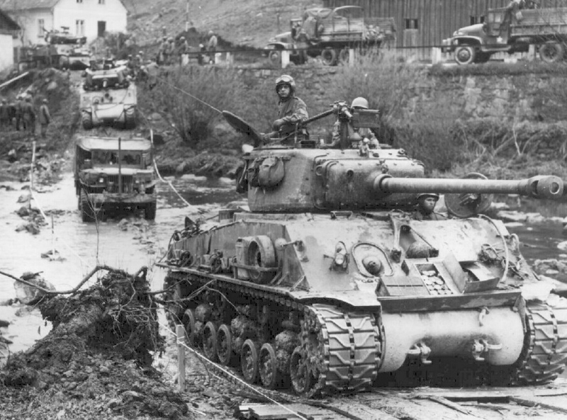
USS America in Vestfjord clearly showing how the mountains would block the line of sight of missile-carrying bombers until they were very close to the target. (USNI Proceedings)

Vestfjord is created by the Lofoten Archipelago that forms the northern side of Ofotfjord at Narvik and extends about 100nm into the North Sea. The dramatic vertical relief provides an excellent radar shadow protecting ships operating in the deep waters close inshore from airborne radars searching from the north. If that were the only trick up the Soviet sleeve, hiding in Vestfjord’s radar shadow would provide extra time for the CVBG’s F-14s to whittle down the attacking bombers before they could achieve line of sight and launch their missiles. That wasn’t, however, the end of the story. In fact, it was just the beginning for me.

Over a period of about three years in the late 1980s, I participated in a number of wargames where this issue came up. As a Soviet Air Forces analyst, I brought a different perspective to the problem. Secretary Lehman was well aware of the threat SNA posed to his CVBGs, but he was undoubtedly unversed on Soviet Air Force (VVS) capabilities and formations, since it would not have been a factor for him until he sent the Navy into Vestfjord

While duking it out with the Navy, I ran into a phenomenon well-known within the wargaming community where the Navy under no circumstances would allow one of their aircraft carriers to be portrayed as being sunk or even seriously damaged. In one exercise, I was told that an attack by 90 bombers had managed to slightly damage one catapult. In another, my pilots had mysteriously mistaken a Royal Navy jump-jet carrier for a US CVN four times its size. After taking major losses on that raid, I nonchalantly told the Blue Navy player that I would whistle up another bomber division (like we “had plenty more where that came from”) and go at it again, tomorrow. He winced and admitted to me that there wasn’t any point because they would never allow me to sink a carrier. I replied that I just wanted him to admit that out loud before I let it go.

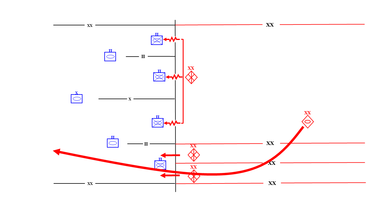
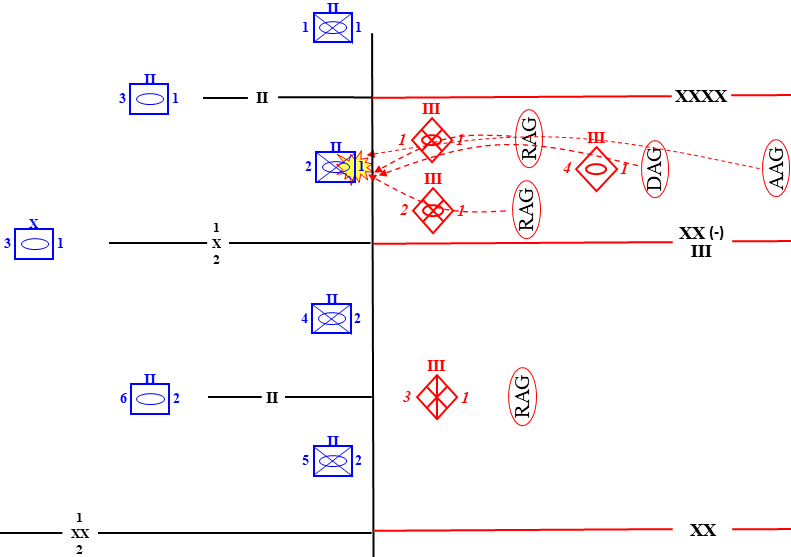
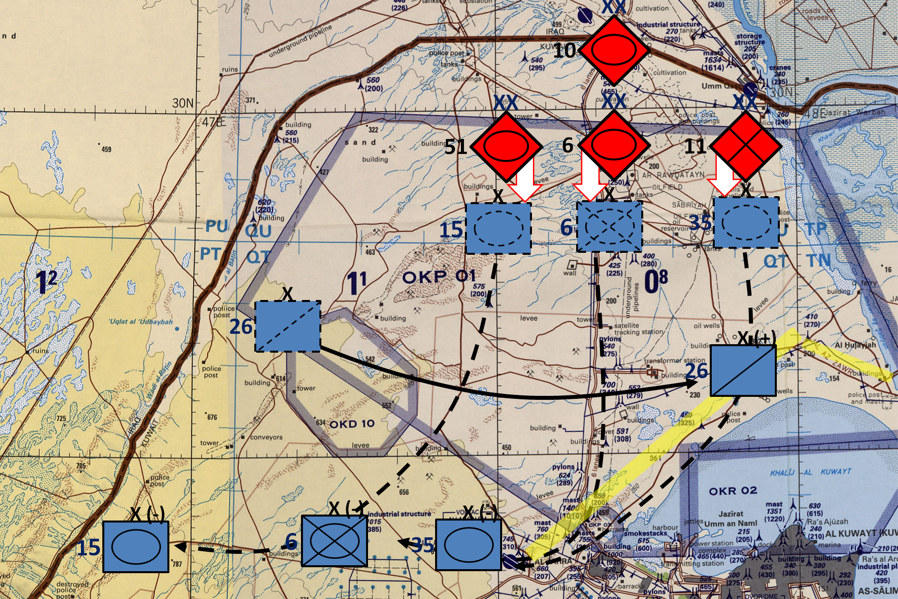
Yellow:  SNA ASCM-carrying bombers fly from bases on and near the Kola, around the North Cape and down the coast of Norway. Large purple circle: Kh-22 300nm launch line. Small purple circle: Kh-22 67nm launch line (reduced by the radar shadow in Vestfjord). Blue: USN F-14 fleet defense fighters push north to intercept the SNA before they can get radar line-of-sight to the CVBG. Red: VVS Bomber Aviation Division uses the mountains to screen its attack on the CVBG.

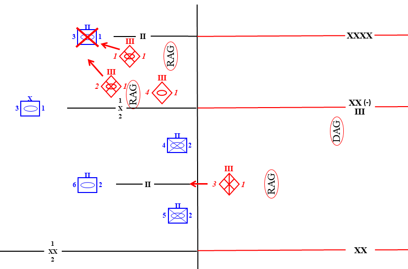
The final showdown came when I was called to the Pentagon and asked to give all the details of my tactics in a mano a mano combat with a Navy officer and a rather large crowd of onlookers. My final plan went like this: I sent a major SNA raid from the north to threaten the two-carrier CVBG hugging the southern slope of the mountains in Vestfjord. My opponent, knowing the broad strokes of my strategy, tried to hold back F-14s in reserve. However, he was quickly cut off by another Navy officer who said that the F-14s would have to “honor the threat” by committing the interceptors against the SNA bombers. 

While the F-14s were tied up 100-200nm north of Vestfjord, I sent in a bomber aviation division with about 90 Su-24/FENCER light bombers armed with a pair of 1,500kg Laser-guided bombs apiece. This force went into Vestfjord in a long trail formation covered by Su-27/FLANKERS. My opponent raised the difficulties of finding the target ships, but I countered that in a trail formation, all the later aircraft need do would be to follow the smoke columns from the fires of shot down aircraft and damaged ships. 

The FENCERS hugged the mountains so that their radars were looking out to sea for the CVBG, while the US radars were trying to pick out FENCERS from the radar clutter of the mountains behind them. What had been sauce for the goose had suddenly become sauce for the gander. The Navy knew from experience that picking out fighter aircraft from the mountains was a nasty challenge. This gave the VVS bombers a real chance to make it through to the target.

While nearly all modern warships lack any kind of significant armor, US Navy aircraft carriers are the exception. The Navy keeps the details close to their chest, but even if they don’t have conventional armor plate like a battleship, the use of fuel and water tankage can create a reasonable facsimile, while the sheer size of a carrier and the compartmentation available ensure that any damage is isolated and kept away from the vital areas of the ship. To do real harm takes a large bomb with real penetrative capability. Both of these are embodied in the 1,500kg bomb. Further, while dropping from low altitude — deck height or lower — the bomb would impact almost perpendicular to the side of the ship, ensuring maximum penetration. Laser guidance wouldn’t add too much to the equation, but it did give me an extra argument to deflect disputes about accuracy. With the bombs detonating inside the ship, there would be no danger from fragging one’s own aircraft and little danger to following planes, as well. A further advantage to dropping from such low altitude would be that it would be nearly impossible to mistake the target carrier with anything else — no other ship would tower over the bombers so they need only steer for the biggest object ahead of them.

Squirm as he might, my opponent was frustrated at every turn. Each idea he came up with was shot down by the onlookers. The Navy observers looked at our little desk-side exercise and could find no way out. They were finally forced to concede that their carriers were not invincible, after all. From that day to this, I haven’t heard the Navy talk about Vestfjord or taking on land-based air. My campaign may not have been what caused the Navy to rethink The Maritime Strategy, but it assuredly provided at least one nail in the coffin.

Naval wargaming is simple and straightforward when compared to wargaming ground combat. Naval warfare lends itself to mathematical fights between weapons systems.  There are little, if any, terrain considerations and all the combatants can be discretely modeled. Further, there is little of the human element to be considered as most of the interactions are, in reality, controlled by computer. In contrast, a land battle has a nearly infinite number of interactions and the human factor is the most important single determinate of defeat — you defeat the enemy by breaking his will to stand his ground — while weapons are merely tools to get inside his head. Elsewhere in this blog, I have stated that I had $40 commercial wargames in my closet that could do a more realistic job than the Pentagon’s million-dollar computer models. The cost factor only grows larger with naval wargames.

Perhaps this is why the US Navy has traditionally invested in wargames: the inherent simplicity, clarity and believable results of naval wargames make them accessible and instructive. After WWII, Fleet Admiral Chester Nimitz was asked if anything surprised him during the battles of the Pacific war. His answer, that only the Japanese use of Kamikaze tactics had not been foreseen and wargamed before the war ever began, is informative on the utility of naval wargaming. The US Naval War College continues to this day to run annual wargames with its students working on fleet problems with real-world relevance. The War College’s own website declared that, “Simulating complex war situations—from sea to space to cyber—builds analytical, strategic, and decision-making skills. Wargaming programming not only enriches our curriculum, but it also helps shape defense plans and policies for various commands and agencies.” Thus saith the Navy. The Air Force would agree. If we can get the Army in on it, we might have something of use to the nation.

[1] Zakheim, Dov S. and Lehman, John (2018) “Lehman’s Maritime Triumph,” Naval War College Review: Vol. 71 : No. 4 , Article 11. Available at: https://digital-commons.usnwc.edu/nwc-review/vol71/iss4/11.

[2] Watkins, James D. Admiral USN, The Maritime Strategy, US Naval Institute Proceedings, January 1986, https://www.usni.org/magazines/proceedings/1986/january-supplement/maritime-strategy-0.

[3] Ibid.

——

His other recent and related articles are:

The Easy Button | Mystics & Statistics (dupuyinstitute.org)

Wargaming 101 – The 40-60-80 Games | Mystics & Statistics (dupuyinstitute.org)

Wargaming 101 – In the Bowels of the Pentagon with J-8 | Mystics & Statistics (dupuyinstitute.org)

Wargaming 101: The Bad Use of a Good Tool | Mystics & Statistics (dupuyinstitute.org)

Wargaming 101: A Tale of Two Forces | Mystics & Statistics (dupuyinstitute.org)

He is doing a presentation at HAAC on Day 2 (Wednesday, Oct. 18) on Wargaming 101: Schedule for the Second Historical Analysis Annual Conference (HAAC), 17-19 October 2023 | Mystics & Statistics (dupuyinstitute.org)


Wargaming 101 – The 40-60-80 Games

Yet another great article from William (Chip) Sayers. First of three that are coming. The conclusions are his. 

——-

Wargaming 101 – The 40-60-80 Games

Shortly after the George H. W. Bush Administration entered office in 1989 a story — probably apocryphal — was making the rounds. In the story, President Bush and the Chairman of the Joint Chiefs of Staff, Admiral Bill Crowe, were on the back nine when the Commander-in-Chief turned to the Chairman and said, “Bill, I want you to gather together our best wargamers and game out some scenarios for the Conventional Forces in Europe talks. I’d like you to look at bringing the two sides down to parity and then do three wargames where one takes the two side’s forces down a further 20% to 80% of baseline parity, a second down to 60% of baseline and finally one at 40%.”

For many years of the Cold War the Conventional Forces in Europe (CFE) talks were on the books, but nobody took them seriously. Then, in the late 1980s, they were suddenly on the front burner with a real chance of yielding results. President Bush wanted us to have credible proposals ready if a breakthrough occurred and in particular, he wanted to thoroughly understand the implications of various possible proposals. The crux of the matter was a question of force-to-space ratios. For 40 years the two sides had sufficient forces to man a continuous line of units from the Baltic Sea to the Swiss Alps. CFE was designed to lessen the chances and consequences of war by radically reducing the forces of both sides. The problem was that no one knew how the character of a war in Europe would change when this was no longer true.

Heading the project was the legendary Huba Wass de Czege, at that time a Colonel about to pin on a general’s star. EUCOM sent its best and brightest to provide the Blue side, DIA was tasked to man the Red team, while J-8 facilitated the games. The plan was for each team to wargame its scenario as many times as possible within the time allotted and note any points of interest.  We quickly began referring to the exercise as the 40-60-80 games. I was assigned to run Red for the 60 game, which turned out to be the most interesting of the three scenarios. COL Wass de Czege instinctively knew this would be the case and he spent the majority of his time with us. The 80% game was too conventional to be very interesting, while the 40% game would be the Wild-West — no structure, too much open-field running to deal with in an organized manner. The 60% game would have the right amount of possibilities with the structure needed to make it work. COL Wass de Czege’s presence was a good gauge for where the real lessons would be learned and the longer the exercise went, the more time he spent with the 60% team.

The Blue Air guy opposing me was a US Air Force officer from EUCOM who had some distinctive ideas about how to use airpower. His main line was that airpower should be used in mass, that rather than parceling it out, one should concentrate to eliminate a target-set in its entirety. Not a bad thought. However, the White Cell controllers found him very persuasive. At one point, he directed a mass air attack on one of my second echelon formations, two Combined Arms Armies lying in wait in the Thüringer Wald. The controller looked at his tables, reached over and dumped all eight divisions in the dead pile. I’m an airpower guy myself, but in my wildest dreams I would never believe that this could happen. Billy Mitchell and Giulio Douhet would have blushed. In other circumstances, I would have been happy to explore Major Airpower’s theories, but I was concerned that his fantasies were going to skew the results of the games and that COL Wass de Czege, as a ground-minded Army officer might not be able to sort this out. I wrote the Colonel a note at the end of the exercise explaining why I was concerned with airpower’s portrayal. In retrospect, however, I doubt I needed to worry about the wool being pulled over COL Wass de Czege’s eyes.

Fortunately, it was during our games that Capt. Alex Zuyev of the Soviet Air Force decided to abscond with one of the USSR’s newest jets and deliver his MiG-29 to Turkey. Major Airpower was called back to Europe in a hurry to help find out what he could about Zuyev’s jet, leaving me free to play the game without an omnipotent air force to fight. Nevertheless, even with my nemesis gone, I still had some systemic problems to overcome.

As I noted in a previous post, the models at that time had a severe bias against the attacker. It was extremely frustrating to be told that an entire Combined Arms Army could be held in check by a single NATO division when I knew I could devise a plan that would make a mockery of such ridiculous assertions.

If the NATO division concentrates to have a realistic chance of holding off a force twice its size, the remaining Soviet divisions easily sweep through the cavalry screen monitoring the defender’s right.

If the NATO division instead spreads out to cover its assigned sector, the Combined Arms Army concentrates to make a breakthrough for its tank division to exploit into the defender’s rear.

In order to make up for such obvious problems, COL Wass de Czege gave me extra forces to work with. The justification for this was that the Soviets did not have to count units east of the Ural Mountains under the terms of the agreement as it then stood.  Eventually, we posited an early movement of these forces — since the Soviets would know when they intended to attack — and had them arrive in time to take part as the second echelon of the operation. It was a bit of a cheat, but a very reasonable one in our estimation. I don’t remember who came up with the idea, whether it was me, someone else, or COL Wass de Czege himself, but it had the full backing of the Colonel, and that’s what mattered.   

My biggest frustration, however, was that my attempts to execute an Air Operation kept ending in miserable failure, with no apparent effect on Blue Air at all. This prompted a very revealing conversation with a White Cell controller. We basically broke open the “black box” of the model and found that the algorithms assumed a single runway 24,000 miles long — essentially encompassing the entire Earth at the equator. Even Fairchild-Republic — maker of the A-10 and a manufacturer reputed to build its aircraft to use the last third of any runway, no matter how long it was — would have to bow to this monstrosity. I was unable to come up with a hack to overcome this problem, but at least knowing how the model was cheating allowed me to conserve resources that I had been wasting pursuing an impossible task.

On our final run-through, I developed a tactic that, if not entirely realistic, was very successful in overcoming some of the model’s bias against the attacker. I attacked with Combined Arms Armies deployed in two echelons. On two or three occasions, I had two CAAs attacking on parallel lines successfully pushing a Blue Corps back until held up by Blue’s defense of a river line. Because I had put extra weight behind this push, there were Blue forces on Red’s flanks, which seemed to the Blue players to be a good thing, but they weren’t counterattacking through those flanks. They hadn’t turned to face inward — apparently, they had their hands full to their direct front — so I turned my second echelon divisions 90⁰ toward either side and attacked into Blue’s rear areas.  My Blue counterpart protested that you can’t just turn on a dime and attack, but now it was my turn to be persuasive. I answered that Patton did it at the Battle of the Bulge and that was what second echelons were for. That argument carried the day. It probably shouldn’t have been that easy — my counterpart was right, armies are unwieldy and have large logistics trains following them around — but the Soviets were structured better for that kind of maneuver and Blue’s defenses had no business being as effective as they were, so I wasn’t too troubled by it.

In COL Dupuy’s Understanding Defeat, he points out that, historically, the single most important factor causing defeat in land combat is the fear in the minds of defending troops that the enemy is on their flank, or worse, in their rear. By hitting Blue in the “joints” between Corps, I was able to force the flanking corps to displace to avoid entrapment. This left open flanks on the targeted corps, which was, in turn, forced to give ground to avoid being enveloped.

My Blue counterpart had no answer for this and so we went from position to position with Red leveraging Blue out of strongpoints with maneuver. I was able to gradually make progress marching to the North Sea in a thrust reminiscent of the France 1940 campaign. My operation culminated just a few kilometers from the sea, but the thin strip of land we didn’t occupy was easily dominated by Red artillery, so I believed we had accomplished our mission in isolating three NORTHAG corps from the rest of NATO’s central front. I was understandably happy with the results. They called it a Blue victory.

COL Wass de Czege considered the events, picked up his notes and headed off to Europe. The Colonel was correct about the relative value of the various scenarios: I peeked in on the other gamers from time to time and the 80% games looked a lot like the usual J-8 affairs, while the 40% games looked a lot like air combat with units zipping around the map to strike a particular point, only to have an enemy unit chase them down as though they were in a dogfight. None of that felt very real to the players, but they were frustrated because they couldn’t come up with a rationale to restrict play to something that seemed more plausible. To me, at its best it resembled nothing so much as operational-level maneuver during the Napoleonic Wars. I made a note of that for future consideration. It would have been interesting to explore that idea, but the 60% games were where the action was and gave rise to the most interesting results.

I don’t know what impact the 40-60-80 games had on the CFE negotiations, but the Conventional Forces in Europe Treaty was soon a reality, and it was nice to feel like I had a piece of that history. Interestingly, the Soviet General Staff tried a gambit to gain as much advantage as they could by proposing that we use their Correlation of Forces methodology to measure force strength. There is no doubt that it would have been a smart move to incorporate qualitative factors as well as quantitative ones in the sorting out of force strength. However, the General Staff had control of the methodology and the scores they proposed for individual pieces of equipment were neither what we would have expected, nor did they look anything like previous Soviet assessments. In short, they were clearly undervaluing their own arms in comparison with the West’s in order to keep an advantage in numbers. We ended up rejecting the use of CoFM in the treaty process, but it proved to be a coup to gain valuable insight into how the Soviets did business. Many of the formulas I use in modeling are a direct result of these exchanges.

Unfortunately, events soured me on the process in an unexpected way. As with most arms treaties, CFE was only possible when circumstances changed such that it was no longer necessary. It was completed with the foundation that the Warsaw Pact countries would remain allies of the Soviet Union when it was clear that wouldn’t actually be the case. Nevertheless, Polish, Czech, East German, Hungarian, Romanian and Bulgarian units were counted as being on the Soviet side of the calculation. It was a bit of an unfairness, but Gorbachev was in such great need of relief, he acceded to it. When the Bush Administration left office after only four years, they were replaced by the Clinton Administration which was heavily criticized for not having a depth of experience in foreign affairs. The CFE Treaty was still new when they took office and their inexperience took its toll.

In 1991, Germany reunified and the General Staff saw six of the former Pact’s best divisions move from the Pact column to the NATO column. They believed they should get some adjustments to compensate. The Clinton Administration ultimately rejected compensation. Then, one by one, other former Pact countries announced their intention to apply for NATO membership. It made no sense that these forces should be counted against the (now) Russian side when they would actually be fighting for NATO. We were holding Moscow to terms that made no sense and were fundamentally unfair, but in a spirit of triumphalism in the 1990s where they wanted to claim the Cold War victory as their own, Clinton’s people danced on the grave of the Soviet Union, believing that Russia would forever be too weak to cause us problems, no matter how just their cause. Or at least not until after a second Clinton term. They rejected major Russian-proposed changes in the treaty. In 1996, when Russia was faced with conflict in the Caucasus region, we did allow an amendment that took into account the fact of what would have been a civil war a few years prior. Moscow believed the US and NATO were using a treaty meant to end the possibility of conflict between the two blocs to interfere with security challenges legitimately within their sphere of interest that had nothing to do with a potential NATO/Pact conflict. Lest I be accused of political bias, the George W. Bush Administration did little better, managing to incense the Russians by building bases in former Pact countries the Russians believed to be in violation of the treaty.

I recently read an opinion piece that ultimately blames our treatment of Russia in the 1990s for the current war in Ukraine. While we should never condone or fail to resist to our utmost the kind of outrageous military action Russia has taken against a sovereign neighbor, we should learn the hard lessons of how unjust actions we take can come back to haunt us years down the road. Putin partially suspended Russia’s participation in the treaty in 2007 and then withdrew entirely in 2015. The Russian strong-man is undoubtedly the worst war criminal to appear in Europe in the last 80 years; nevertheless, he didn’t spring onto the world stage fully formed. We should soberly reflect on our responsibility in making him what he is today.

——————-

Unstructured Comments on “The Relationship of Battle Damage to Unit Combat Performance”

Thanks to Russell1200 (see comments to Count of Opposing Forces | Mystics & Statistics (dupuyinstitute.org)), I now found out about a report “The Relationship of Battle Damage to Unit Combat Performance” by Leonard Wainstein of IDA prepared back in April 1986. Both the report and Wainstein are unknown to me.

The abstract of the report says

The purpose of this study is to investigate the historical basis for the assumption that a military formation will cease to be effective after having lost a pre-ordained percentage of its strength. Battles from the First World War to the 1982 Falklands campaign are reviewed for insight into the validity of this assumption.

The effect of heavy battte damage on units has been both variable and unpredictable. There is a relationship between losses and the continued willingness to fight, but it defies precise definition. So long as some men in the formation continue to fight as an organized entity, either in attack or defense, for whatever reason, the formation they represent cannot be termed ‘ineffective.”


My notes made while reading it:

  1. Page v: Contents: section on earlier studies references ORO report of 1954 (known to me… the Dorothy Clark report on Breakpoints) and an RAC report of 1966 (not known to me).
  2. Page 1: “The battle cases cited run from army level to battalion level, from single day engagements to those lasting several months” – my bias is to collect and analysis data based upon the same level of combat, i.e. division-level, battalion-level, etc.
  3. Page 1: Only 54 actions were examined (this seems small) and “only 11 represent cases where a formation collapsed, surrendered, was repulsed, was stalemated, or had to be taken out of the line after suffering some degree of damage.” (this seems like a really small sample).
  4. Page 2: “Colonel Trevor N. Dupuy, in describing the 1973 Middle East War, has written ‘The human element has always been important in war, and despite the technology available to both sides, the human element was undoubtedly the most significant feature in this war.’ The same comment could obviously be made about all the actions described in this paper.”
  5. Page 3: “There is no agreement among national armies, combat commanders, military historians or defense analysts as to the point when battle damage renders a formation impotent.”
  6.  Pages 1-5, Summary: This is worth reading in its entirety.
  7. Page 6: “The modeling community have developed a set of formulae for use in this determination, but it is not clear to what extent these formulae reflect actual battle experience.” (stated in 1986… pretty certain the “modeling community” has not taken significant corrective action).
  8. Page 8: Paragraph on perceived resistance is interesting.
  9. Pages 1-10: No mention of artillery.
  10. Page 11: “Despite the interest in and significance of the subject, relatively little research has been done across the years on casualty-effectiveness relationships.”
  11. Pages 11-12: Description of the Dorothy Clark 1954 ORO report, measuring 44 battalions. To quote Clark “the statement that a unit can be considered no longer combat effective when it has suffered a specific casualty percentage is a gross oversimplification not supported by combat data.”
  12. Pages 12-13: Description of Robert Best 1966 RAC report.
  13.  Page 23: Trevor Dupuy quoted again.
  14. Page 24: “Oriental fanaticism.”
  15. Page 44: HERO report from 1967 is referenced (HERO became TDI).
  16. Page 69: Trevor Dupuy is referenced.
  17. Page DL-2: A copy of this report went to CAA (Concepts Analysis Agency, now Center for Army Analysis).
  18. Page DL-3:  A copy went to HERO. I was there in 1987, do not recall seeing this report.

The IDA report is here: TheRelationshipBetweenBattleDamageAndCombatPerformance.


A few related past posts:

Count of Opposing Forces | Mystics & Statistics (dupuyinstitute.org)

Breakpoints | Mystics & Statistics (dupuyinstitute.org)

Historians and the Early Era of U.S. Army Operations Research | Mystics & Statistics (dupuyinstitute.org)

Advance Rates in Combat

M4A3E2

Advance Rates in Combat:

                Units maneuver before and during a battle to achieve a more favorable position. This maneuver is often unopposed and is not the subject of this discussion. Unopposed movement before combat is often quite fast, although often not as fast as people would like to assume. Once engaged with an opposing force, the front line between them also moves, usually moving forwards if the attacker is winning and moving backwards for the defender if he is losing or choosing to withdraw. These are opposed advance rates. This section is focused on discussing opposed advance rates or “advance rates in combat.”

            The operations research and combat modeling community have often taken a short-hand step of predicting advance rates in combat based upon force ratios, so that a force with a three-to-one force ratio advances faster than a force with a two-to-one force ratio. But, there is not a direct relationship between force ratios and advance rates. There is an indirect relationship between them, in that higher forces ratios increased the chances of winning, and winning the combat and the degree of victory helps increase advance rates. There is little analytical work that has been done on this subject.[1]

            Opposed advance rates are very much influenced by 1) terrain, 2) weather and 3) the degree of mechanization and mobilization, in addition to 4) the degree of enemy opposition. These four factors all influence what the rates will be.

            In a study The Dupuy Institute did on enemy prisoner of war capture rates, we ended up coding a series of engagements by outcome. This has proven to a useful coding for the examination of advance rates. Engagements codes as outcomes I and II (limited action and limited attack) are not of concern for this discussion. The engagement coded as attack fails (outcome III) is significant, as these are cases where the attacker is determined to have failed. As such they often do not advance at all, sometimes have a very limited advance and sometimes are even pushed back (have a negative advance). For example, in our work on the subject, of our 271 division-level engagements from Western Europe 1943-45 the average advance rate was 1.81 kilometers per day. For Eastern Europe in 1943 the average advance rate was 4.54 kilometers per day based upon 173 division-level engagements.[2] These advance rates are irrespective of what the force ratios are for an engagement.

            In contrast, in those engagements where the attacker is determined to have won and is coded as attacker advances (outcome IV) the attacker advances an average of 2.00 kilometers in the 142 engagements from Western Europe 1943-45. The average force ratio of these engagements was 2.17. In the case of Eastern Europe in 1943, the average advance rate was 5.80 kilometers based upon 73 engagements. The average force ratio of these engagements was 1.62.

            We also coded engagements where the defender was penetrated (outcome V). These are those cases where the attacker penetrated the main defensive line of the defending unit, forcing them to either withdraw, reposition or counterattack. This penetration is achieved by either overwhelming combat power, the end result of an extended operation that finally pushes through the defenses, or a gap in the defensive line usually as a result of a mistake. Superior mechanization or mobility for the attacker can also make a difference. In those engagements where the defender was determined to have been penetrated the attacker advanced an average of 4.12 kilometers in 34 engagements from Western Europe 1943-45. The average force ratio of these engagements was 2.31. In the case of Eastern Europe in 1943, the average advance rates was 11.28 kilometers based upon 19 engagements. The average force ratio of these engagements was 1.99.

            This clearly shows the difference in advance rate based upon outcome. It is only related to force ratios to the extant the force ratios are related to producing these different outcomes.


            Also of significance is terrain and weather. Needless to say, significant blocking obstacles like bodies of water, can halt an advance and various rivers and creeks often considerably slow them, even with engineering and bridging support. Rugged terrain is more difficult to advance through and easier to defend and delay then smoother terrain. Closed or wooded terrain is more difficult to advance through and easier to defend and delay then open terrain. Urban terrain tends to also slow down advance rates, being effectively “closed terrain.” If it is raining then advance rates are slower than in clear weather. Sometimes considerably slower in heavy rain. The season it is, which does influence the amount of daylight, also affects the advance rate. Units move faster in daylight than in darkness. This is all heavily influenced by the road network and the number of roads in the area of advance.

            No systematic study of advance rates has been done by the operations research community. Probably the most developed discussion of the subject was the material assembled for the combat models developed by Trevor Dupuy. This included addressing the effects of terrain and weather and road network on the advance rates. A combat model is an imperfect theory of combat.

            Even though this combat modeling effort is far from perfect and fundamentally based upon quantifying factors derived by professional judgment, tables derived from this modeling effort have become standard presentations in a couple of U.S. Army and USMC planning and reference manuals. This includes U.S. Army Staff Reference Guide and the Marine Corps’ MAGTF Planner’s Reference Manual.[3]

The original table, from Numbers, Predictions and War, is here:[4]


STANDARD (UNMODIFIED) ADVANCE RATES


                                                                                    Rates in km/day

                                                Armored          Mechzd.          Infantry           Horse Cavalry

                                                Division           Division           Division           Division or

                                                                                                or Force           Force

Against Intense Resistance

    (P/P: 1.0-1.1O)

Hasty defense/delay                4.0                   4.0                   4.0                   3.0

Prepared defense                    2.0                   2.0                   2.0                   1.6

Fortified defense                     1.0                   1.0                   1.0                   0.6


 Against Strong/Intense Resistance

    (P/P: 1-11-125)

Hasty defense/delay                5.0                   4.5                   4.5                   3.5

Prepared defense                    2.25                 2.25                 2.25                 1.5

Fortified defense                     1.25                 1.25                 1.25                 0.7


Against Strong Defense

    (P/P: 1.26-1.45)

Hasty defense/delay                6.0                   5.0                   5.0                   4.0

Prepared defense                    2.5                   2.5                   2.5                   2.0

Fortified defense                     1.5                   1.5                   1.5                   0.8


Against Moderate/Strong Resistance

    (P/P: 1.46-1.75)

Hasty defense                         9.0                   7.5                   6.5                   6.0

Prepared defense                    4.0                   3.5                   3.0                   2.5

Fortified defense                     2.0                   2.0                   1.75                 0.9


Against Moderate Resistance

    (P/P: 1.76-225)

Hasty defense/delay                12.0                 10.0                 8.0                   8.0

Prepared defense                    6.0                   5.0                   4.0                   3.0

Fortified defense                     3.0                   2.5                   2.0                   1.0


Against Slight/Moderate Resistance

    (P/P:2.26-3.0)

Hasty defense/delay                16.0                 13.0                 10.0                 12.0

Prepared defense                    8.0                   7.0                   5.0                   6.0

Fortified defense                     4.0                   3.0                   2.5                   2.0


Against Slight Resistance

    (P/P: 3.01-4.25)

Hasty defense/delay                20.0                 16.0                 12.0                 15.0

Prepared defense                    10.0                 8.0                   6.0                   7.0

Fortified defense                     5.0                   4.0                   3.0                   4.0


Against Negligible/Slight Resistance

    (P/P:4.26-6.00)

Hasty defense/delay                40.0                 30.0                 18.0                 28.0

Prepared defense                    20.0                 16.0                 10.0                 14.0

Fortified defense                     10.0                 8.0                   6.0                   7.0


Against Negligible Resistance

    (P/P: 6.00 plus)

Hasty defense /delay               60.0                 48.0                 24.0                 40.0

Prepared/fortified defense      30.0                 24.0                 12.0                 12.0


*Based on HERO studies: ORALFORE, Barrier Effectiveness, and Combat Data Subscription Service.

** For armored and mechanized infantry divisions, these rates can be sustained for 10 days only; for the next 20 days standard rates for armored and mechanized infantry forces cannot exceed half these rates.


                This is a modeling construct built from historical data. These are “unmodified” rates. The modifications include: 1) General Terrain Factors (ranging from 0.4 to 1.05 for Infantry (combined arms) Force and from 0.2 to 1.0 for Cavalry or Armored Force, 2) Road Quality Factors (addressing Road Quality from 0.6 to 1.0 and Road Density from 0.6 to 1.0), 3) Obstacles Factors (ranging from 0.5 to 0.9 for both a River or steam and for Minefields), 4) Day/Night with night advance rate one-half of daytime advance rate and 5) Main Effort Factor (ranging from 1.0 to 1.2). These last five sets of tables are not shown here, but can be found in his writings.[5]


[1] The most significant works we are aware of is Trevor Dupuy’s ORALFORE study in 1972: Opposed Rates of Advance in Large Forces in Europe (ORALFORE), (TNDA, for DCSOPS, 1972); Trevor Dupuy’s 1979 book Numbers, Predictions and War; and a series of three papers by Robert Helmbold (Center for Army Analysis): “Rates of Advance in Land Combat Operations, June 1990,” “Survey of Past Work on Rates of Advance, and “A Compilation of Data on Rates of Advance.”

[2] See paper on the subject by Christopher A. Lawrence, “Advance Rates in Combat based upon Outcome,” posted on the blog Mystics & Statistic, April 2023. In the databases, there were 282 Western Europe engagements from September 1943 to January 1945. There were 256 Eastern Front engagements from February, March, July and August of 1943.

[3] See U.S. Army Staff Reference Guide, Volume I: Unclassified Resources, December 2020, ATP 5-0.2-1, pages xi and 220; and MAGTF Planner’s Reference Manual, MSTF pamphlet 5-0.3, October 2010, page 79. Both manuals include a table for division-level advances which is derived from Trevor Dupuy’s work, and both manuals contain a table for brigade-level and below advances which are calculated per hour that appear to also be derived from Trevor Dupuy’s division-level table. The U.S. Army manual gives the “brigade and below” advance rates in km/hr while the USMC manual, which appears to be the same table, gives the “brigade and below” advance rates in km/day. This appears to be a typo.

[4] Numbers, Predictions and War, pages 213-214. The sixth line of numbers, three numbers were changes from 1.85 to 1.25 as this was obviously a typo in the original.

[5] See Numbers, Predictions and War, pages 214-216.


The actual paper this was drawn from is here: Advance Rates in Combat

Wargaming 101 – In the Bowels of the Pentagon with J-8

Another great William “Chip” Sayers article on wargaming. 


Wargaming 101 – In the Bowels of the Pentagon with J-8

I had been a Soviet Military Aviation analyst for DIA for only a few weeks when a friend from my previous life in the Air Force Reserve Intelligence program invited me to accompany him to the Pentagon to observe a wargame being conducted by J-8, the Joint Staff’s Force Requirements directorate.  The J-8 was basically “wargame central” for the Pentagon, using this tool in various forms to evaluate the impact of various proposed force structure changes on the warfighting abilities of the US military.  In this case, the wargame “command post” was dominated by a floor to ceiling map of NATO’s Central Front with small cardboard chits representing units stuck to the clear acetate covering.  One glance was sufficient to tell me all I needed to know:  the units were in a solid line one-deep stretched from the Baltic Sea to the Alps.  It was 1915 all over again.  Not the most auspicious beginning to 10-years of playing Red Cell in J-8 wargames, but I have to admit it got a lot more interesting from there.

One of my more interesting encounters with J-8 was with regard to an exercise known as “Competitive Strategies.”  The brainchild of Senator — and later Vice-President — Dan Quayle, Competitive Strategies was designed identify and implement ideas that would pit enduring US strengths against enduring Soviet weaknesses.  Senator Quayle, at that time considered a true wunderkind  and the smartest person in the Senate, believed that too often the US was pitting strength against strength — a contest the US could not win — and wanted to engage in what would today be referred to as “asymmetric warfare” that the USSR could not match.  For example, pushing technological warfare beyond what the Soviet industrial base could compete with.

J-8 scoured the Pentagon for ideas, then sent them to the intelligence community to be vetted.  I had missed out on Competitive Strategies I, which took place shortly before I arrived at DIA, but was there for Competitive Strategies II and III.  In the first round, a number of ideas were kicked around, but apparently none were found suitable.  In CS II, I was chosen to be on a board that considered a proposal to counter Soviet air operations (lower case).  The Soviet Air Operation (upper case) was a stratagem the Soviet General Staff came up with when they realized that upwards of half of NATO’s combat power resided in their air forces.  The Air Operation was a preplanned series of strikes intended to deny NATO its airpower advantage by destroying NATO’s air assets on the ground before they could be employed.  This meant that the Air Operation, and the initial ground operations as well, would fire the first shots of WWIII.  I was known to be well versed in the Soviet Air Operation — thus my invitation as a relatively junior analyst to serve on the board — and was not pleased with the proposal.  It seemed inordinately expensive, technologically doubtful, and unlikely to yield the desired impact.  The proposal involved creating a force of ground-launched tactical cruise missiles targeted on virtually every Hardened Aircraft Shelter (HAS) on every Soviet and Warsaw Pact airfield in the East Bloc countries.  These missiles would be fired at the outset of hostilities to catch the enemy aircraft on the ground and destroy them before they could take to the air.

The gentleman who served as our chairman was a good and knowledgeable analyst, but I felt at the time was too prone to “go along and get along.”  We met on a Friday and he proposed to rubber-stamp the proposal and let it go because, “It’s what they want.”  We agreed to meet again on Monday to decide the matter.  As I said, I was young and fairly inexperienced in the way of bureaucracy and chaffed at approving an idea I believed was fatally flawed.  First, the idea proposed creating a sizable force above and beyond the existing force structure, clearly a very expensive proposition.  There were probably an average of 36 to 45 HAS on each of 20-30 airfields on NATO’s Central Front, alone.  That’s 720-1,350 missiles on 180-340 launch vehicles, if they piggy-backed on the similar Ground-Launched Cruise-Missile deployment under the Intermediate-Range Nuclear Forces scheme.  The GLCM force as deployed reached a total of 120 GLCM Transporter Erector Launcher vehicles — each with four missiles — in 22 flights of about 69 airmen, each.  This proposed anti-HAS force would have been potentially three times larger — a very significant investment in force structure above and beyond that already fielded.

Worse, it was highly unlikely that the anti-HAS force would accomplish its intended mission.  The Soviets were all about preempting NATO in order to limit the damage to their own forces and infrastructure, while it was almost inconceivable that NATO would fire the first shot in any credible scenario.  NATO was greatly outnumbered in virtually every category of military equipment and personnel, and starting on the offensive was fairly universally recognized as a death-wish, given the advantages of the defender.  More to the point, getting unanimous consent from all of NATO’s member countries to start a war — regardless of the provocation — was laughable.  Even if one could conceive of a scenario where all the members would agree, the time expended in reaching a decision and promulgating it through the system would ensure that the Soviets — who had thoroughly penetrated NATO’s command structure — would have seized the initiative and launched a preemptive strike long before NATO was ready to move.  This being the case, the Soviets would have gotten the first shot in by launching the Air Operation before the anti-HAS force was ready to go into action.  When the cruise missiles arrived at their targets, they would find the HAS either empty or filled with second-line jets to replace the first-line units which would have recovered at dispersal locations away from their main bases.

Being young and inexperienced, I decided to spend my weekend writing my own substitute proposal, which emphasized doctrinal changes designed specifically to answer the Air Operation.  I had spent a reserve tour working on recreating the AO using individual aircraft on a time schedule, so I believed I had some insight on what the strengths and weaknesses were in the operation.  My proposal was more about where and how to fight, vice buying a whole new category of weapon and the infrastructure to support it.  On Monday morning, I handed out my counter-proposal — Countering the Soviet Air Operation — to the other board members.  After reading it, they voted to adopt it in place of the original proposal and send it forward as our recommendation.

A year or so later, I had the opportunity to host and chair an interagency panel to vet proposals for CSIII.  Over 30 years later, the only proposal I remember was one that proposed to raise several divisions of Marines who would invade the Crimean and Kamchatka peninsulas and cause the fall of the Soviet empire because, as everyone knew, the post-WWII Soviets could not abide by the loss of even a single square centimeter of Soviet territory.  Needless to say, that proposal failed to make the cut.  In fact, such was the disconnect between “Blue” strategists and “Red” doctrine that we could not in good conscience give a thumbs up to any submitted proposal.  Nevertheless, it was a fun, if fruitless, endeavor.  Was Competitive Strategies a completely dry hole?  Had the Soviet Union survived longer, I’m sure it would have proven its worth.  As it was, I was later told that there was at least one proposal adopted through the process.  However, modesty forbids me to talk about it further…

Another interesting J-8 wargame I participated in was a NATO exercise in the late 1980s.  My office was directed to supply a “Red Air” commander and I was selected mainly because the game was scheduled to run over the Thanksgiving holiday that year and I was still fairly junior in the office.  In order to save time, it was decided that we would piggy-back on another wargame that was run every year by another organization.  The did the preliminaries and the first three days of combat, and we would take over from there, starting our game on D+3.

Unfortunately, the folks that had run Red Air had no concept of the Soviet Air Operation, what they would target, or how they would fight.  Their model claimed the Soviet side had lost 800 aircraft in three days and accomplished nothing while doing so.  The losses were excessive, but had they been sacrificed achieving some important goal, that would be one thing.  To simply throw them away like so many target drones was ludicrous.  Red Ground had not fared much better.  They were held to an advance of less than ten kilometers across the length of the front — an inconceivably small movement.  The Soviets could practically have tripped and fallen that far forward.  Any model that could produce such results should have automatically been suspect.

Our overall Red commander was an expert at NATO bureaucracy, but knew very little about how the Soviets would fight.  Despite the team’s protests, he insisted on fighting the Red side according to  MC 161 NATO’s Strategic Intelligence Estimate.[1]  MC 161 was supposed to be NATO’s assessment of the threat, but each NATO country insisted on having the final say on how the threat to them would look.  After the document was compiled and approved, it was used to by the various Ministries of Defence to justify their military budgets.  The upshot was that each country had to have a goodly slice of the threat, whether or not it made sense within the scope of Soviet doctrine.  For instance, during this game, I was instructed to come up with a Soviet Air Force threat to Portugal so that the Portuguese military could play.  I dutifully came up with a scheme to send Tu-95/BEAR bombers along a circuitous route across North Africa to hit a NATO target in Portugal only to be told they had been spotted a thousand nautical miles out and swatted down like flies.  I’m pretty sure those weren’t Portuguese Air Force A-7P attack jets that did in the Bears.  The upshot was that NATO had the Soviets attacking everywhere and concentrating nowhere, thus dissipating their forces and chances for success — precisely the opposite of Soviet doctrine.

As it happened, our overall Red commander suffered a health issue and I moved into his position.  I immediately moved to reconfigure the Soviet attack into something much more akin to their actual doctrine.  After having run three practices according to MC 161, the “Blue” players were unprepared for what hit them — they undoubtedly felt sucker-punched.  To be fair, Blue’s big move had not been a part of the practice runs, either so both sides were confronted with surprises. 

The final plan with fixing attacks (screw-type arrows) to pin three NORTHAG Corps in place while the Northernmost corps was hit with overwhelming force.  The critical moment occurred whenSACEUR ordered a rearward passage of lines to save the corps sector.

The original plan had the Soviets attacking in proportionate attacks all along the front.  The big change I made for Red’s ground offensive was to concentrate forces against the weakest of the NATO corps, while making lower-odds attacks to fix the other forces in place.  Since NATO exercises always assumed a Soviet/Pact invasion, the tools used by white (control) cells developed in a way that were inherently biased to favor the defense.  This bias insinuated itself into the programing of computers that were eventually used to adjudicate results to the extent that the attacker had to overwhelm the defender to make any ground at all.  Witness the beginning of this exercise where in the first three days of fighting, Red forces made less than 10km in the advance.  Our final plan set up an attack so overwhelming that even the computer could not deny a Red victory.  Even that victory was limited such that the Supreme Allied Commander Europe (SACEUR) was able to order a corps-level rearward passage of lines to introduce a fresh defending force in that sector. 

A rearward passage of lines has an unengaged, fresh force set up defensive positions to the rear of the force to be relieved while it is still delaying the enemy.  When the relieved force is pushed back to the relieving force’s new defensive positions, the relieved force slips through the lines at prearranged points with the relieving force taking up responsibility for the sector.  It is one of the most complex and difficult of military maneuvers, and for a brief time, twice the normal amount of defenders are squeezed into the attacker’s line of fire.  To help minimize the risk, SACEUR ordered a fleet of reserve combat aircraft brought in from the UK and other rear bases to cover the maneuver.

One of the key factors in the Red victory came from an unlikely source.  Having failed to do the Soviet Air Operation in the first three days of war, the previous crew left a lot of tools lying around unused.  It so happens that Blue’s movement of aircraft was noted by Red intel and was particularly vulnerable to a belated Air Operation as the aircraft were being staged through auxiliary bases without aircraft shelters.  It would take a little explaining to the control cell, but fortunately, I was on good terms with their leader, having hosted him at my house for an evening of hobbyist wargaming before the exercise.  It turns out that he was one of my all-time favorite game designers, so we had a common language to use.  One of the interesting things I found out was that the program J-8 was using did not explicitly model airbase attacks, and in particular, runway attacks.  I explained to my friend how the Air Operation would work and some of the tricks involved, and he proposed work-arounds to give me realistic results.  Therefore, at the moment that NATO was at its most vulnerable, all of the air cover over the Schwerpunkt turned out to be Red, not the Blue that was intended.  Faced with a catastrophe, Blue’s moves were ludicrously out of touch, the perfect example of Col. John Boyd’s Observe, Orient, Decide, Act-loop going unrecoverably out of cycle.  Everything they did was increasingly out of synch with the reality on the ground and only made matters worse.  The exercise ended with a huge, smoking hole where NORTHAG used to be.

While SACEUR came to the Red Cell to shake our hands, thank and congratulate us on a successful exercise, I am doubtful he was much concerned about what happened on the map as the point was to stimulate conversation among the top NATO leadership.  However, the exercise was never repeated, so I might have gone a tad overboard in delivering a “realistic” enemy.


[1] See NATO STANDARD AJP-5 ALLIED JOINT DOCTRINE FOR THE PLANNING OF OPERATIONS Edition A Version 2 MAY 2019, NORTH ATLANTIC TREATY ORGANIZATION ALLIED JOINT PUBLICATION, Published by the NATO STANDARDIZATION OFFICE (NSO) © NATO/OTAN; https://www.coemed.org/files/stanags/01_AJP/AJP-5_EDA_V2_E_2526.pdf  Accessed 12Feb23.

Wargaming 101: The Bad Use of a Good Tool

Another William “Chip” Sayers article. He has done over a dozen postings to this blog. Some of his previous postings include:

Wargaming 101: A Tale of Two Forces | Mystics & Statistics (dupuyinstitute.org)

A story about planning for Desert Storm (1991) | Mystics & Statistics (dupuyinstitute.org)


Wargaming 101:  The Bad Use of a Good Tool

In the mid to late 1980s, an office tasked with analysis and support concerning our NATO allies used Col. Dupuy’s Quantified Judgement Model (the predecessor of the TNDM) in analyzing the probable performance of NATO forces in the event of a conventional war in Europe. Why their counterpart for Soviet/Warsaw Pact countries, did not buy the QJM nor, apparently, participate in this analysis is unknown. The NATO office set out to do a series of analytical papers on the various NATO corps areas, presumably producing a study for each. Only two studies were published, one for each of two of the Corps that were considered NATO’s weakest. 

To understand how this project was conceived and designed, one needs to be familiar with NATO’s basic force structure for the Cold War. NATO’s Central Region was divided into eight national corps “slices.” The British, Dutch and Belgians each contributed one corps while the US provided two (plus a third that could rapidly deploy manpower from CONUS to fall in on prepositioned equipment) and the Germans three. Stacked together, they made up what was commonly referred to as the “layer cake” by those who saw fundamental weakness in this scheme. 

By assigning each nation a front-line area to defend, all of NATO would be involved from the outset, with no room for political maneuver — less resolute nations would be locked in from the start of the conflict. However, this meant that certain corps sectors were defended by suspect armies, creating opportunities for Soviet forces to breakthrough NATO’s main line of resistance and romp through their vulnerable and lucrative rear areas. NATO partially compensated by narrowing some of the weaker corps’ sectors and assigning more frontage to the stronger corps. Nevertheless, many believed this scheme of defense was more about politics and less about warfighting.

From North to South, NATO’s Northern Army Group (NORTHAG) consisted of I Netherlands (NE) Corps, I German (GE) Corps, I British (UK) Corps and I Belgian (BE) Corps. Immediately South of NORTHAG was NATO’s Central Army Group (CENTAG), made up of III GE Corps, US Seventh Army (V US Corps and VII US Corps) and II GE Corps.

The first thing one might notice about this arrangement of national corps sectors is that they vaguely look like cylinders of an in-line engine and would take little imagination to envision the Warsaw Pact forces as pistons attempting to push through those cylinders. In fact, a lot of 1980s Pentagon-type wargaming was done based on this idea. Of course, there are a couple of problems inherent to this concept. First, the Soviets knew there would be boundaries between the NATO corps, and that those boundaries would be natural weak points in the defensive scheme. How does one replicate that in a piston-based model? Second, it does not allow for maneuver, particularly across corps boundaries, but also within the “cylinder.” One rather expensive system by a beltway bandit contractor attempted to compensate in their piston-based model by using some mathematical modification, but this never proved convincing. Piston-based models were imminently tempting, but they were a trap that should never have been used. The first time I encountered one, I commented to a friend that I had better wargames in my closet at home, and they cost a whole lot less: $40, vice $1,000,000. I could have saved the Pentagon a lot of money on that one.

Unfortunately, the analysts in question fell for the piston trap. With apparently little or no input from their Soviet counterparts, they chose a relatively weak Soviet Combined Arms Army to act as an attacker, lined them up in the cylinder and sent them off in what was conceptually a simple frontal attack.

Feeding this rather simplistic scenario into the QJM gave results that were satisfying, but would have been suspect to analysts familiar with Soviet Army doctrine. In essence, the study’s analysts “found” that a weak NATO corps could successfully hold off a Soviet CAA and, by implication, a strong corps might be able to defeat or even successfully counterattack its Soviet assailant. A recent QJM run of this scenario resulted in an advance rate of only 2.7km per day — approximately 10% of Soviet planning norms. The second study had similar results, reinforcing their views. Both studies were beautifully done with color graphics and lavish detail. I was green with envy. My agency should have done one of these studies for each NATO corps, and they should have been done with much more understanding of how both sides would fight. It was a huge missed opportunity.

Unfortunately, these beautiful studies were foundationally flawed and would have misled had they gained traction. I don’t know why they failed to do that, whether it was patently obvious to Soviet analysts that the studies were wrong, whether no one believed in the QJM, or whether they were a tree falling in a forest with no one to hear. Most likely, they simply hit the street too late to be of interest, because the Warsaw Pact was crumbling and taking the Soviet threat to Europe off the board.

The studies’ analysts made several fundamental errors in setting up their scenarios.  First and foremost, they misjudged the threat they were working against. They posited that the weakest corps in NATO would face off against a weak Combined Arms Army with no reinforcement. Nothing could have been further from the truth. The Soviets knew NATO’s strengths and weaknesses — in some cases, apparently better than NATO itself — and had no intention of pitting weakness against weakness. Take a look at the following illustration, typical of the time and with at least a fair understanding of how the Soviets planned to go to war:

Note the thrust through Göttingen. Clearly, this is the main effort for the entire Western TVD (Theater of Military Operations). Rather than attack with a weak CAA, the Soviets would likely have thrown the full weight of their operation at the Schwerpunkt of the weak NATO corps. Not only would the strongest Soviet CAA made the attack, it would have had the assistance of second echelon artillery brigades whose parent armies were yet committed, their organic air support, and the lion’s share of Front supporting assets, as well — a very formidable force, indeed.

A second major mistake the studies’ analysts made was assuming that the Soviet thrust would have respected NATO corps boundaries. Take another look at the illustration, above. The main thrust is clearly divided between two armies. It was typical of Soviet battle planning that two adjacent armies would plan their breakthroughs to be side-by-side to take advantage of the potential for sharing supporting assets, to double the size of the breakthrough, and to add to the enemy’s confusion and dislocation by presenting a perplexing attack exploiting seams between defending corps. These two mistakes are why I surmise that Soviet analysts didn’t participate in the study. Surely, they would have corrected these errors.

These were problems with the scenario, but the modeling they did was fatally flawed in itself. If one is examining an operation at a particular level, one must use sub elements of that level to do a proper exploration. To simply feed the model two sides and press “start” is to believe in magic — that the model is able to sort out how the units would interact. By simply dumping the two sides into the model and pressing “start,” they were modeling a simple frontal attack circa 1915. To get legitimate results, the analysts must contribute more than this. 

The QJM was scaled to division/day operations, which means it works best if the maneuver elements are divisions. It works well with brigades/regiments and even down to the battalion and company levels. If the analysts wanted to explore the operations of a corps, they should, at a minimum, have laid out a division-level defense. Better yet, they should have taken it down to the brigade-level to account for nuance. Certainly, the model would have had no problem doing so and the results obtained would have been far more believable. Yet they did their simulation at the corps level, with no maneuver attempted. It’s no wonder they got such desultory results. Unfortunately, the analysts didn’t understand this.

So, how should the QJM have been used to better shed light on the reality of the situation? Clearly, the studies’ analysts needed a better order of battle for the Soviet side. Soviet analysts should have provided that for them, and it assuredly would have been more formidable than what they came up on their own. Further, they needed Soviet experts to set up a better attack for them. It should have included a mix of low-combat power attacks designed to fix enemy forces in place over wide frontages, and high-combat power attacks over a limited frontage to achieve the actual penetration of enemy defenses. Finally, they should have set up a detailed defense. Generically, it would have looked something like this:

A generic NATO corps of two mechanized divisions and a mechanized brigade in a “2 up, 1 back” defensive posture.  

In terms of raw combat power, the CAA with no reinforcement had a 2:1 advantage of the defending corps. Modifying the defenders for posture and terrain and other operational factors drove this down to a 1.6:1 advantage.

Our NATO corps defended approximately 40km of frontage divided between two mechanized divisions. One brigade of the northernmost division defended relatively open ground and was the target of the Soviet breakthrough attack. The second brigade of that division and the entire southern division occupied defensive positions on rougher ground and would therefore be subject to economy of force fixing attacks. The two divisions together had eight front-line battalions in the main line of resistance, each on a defensive frontage of 5km — a fairly comfortable force-to-space ratio. Unfortunately for NATO, the Soviet’s breakthrough frontage norms could be compressed to as little as 4km for a division with two regiments leading. In this case, that could mean a single defending battalion would receive the full weight of an entire attacking division, plus its attached fire support means. This might be one thing with a modern, well-equipped, well-trained, and well-supported corps. However, the NATO corps in question was none of these things.

The Soviet Army immediately to the north of our CAA had a more challenging enemy to overcome, so it chose to make its breakthrough attack through the northernmost battalion sector of our weak NATO corps. By aligning these two attacks on their common border, the Soviets ended up with a breakthrough zone of 10km and were able to share resources and targets.

A strictly numerical accounting of the breakthrough would show two defending companies of APC-mounted infantry at the line of contact with a third in depth, behind them. This array would be hit with a short but supremely violent “hurricane” barrage of over 400 artillery tubes and rocket launchers. This would be achieved by using the division’s organic assets (144 systems), plus the assets of an unengaged second-echelon division (144 systems), plus the CAA’s organic artillery brigade (72 systems — an unengaged a second-echelon army’s artillery brigade could provide support to another attacking division), plus assets from the CAA’s MRL regiment (54 systems).

From the unclassified DIA report, DDB-1130-8-82 Soviet Front Fire Support 15Dec81.

400 tubes firing at an average rate of five rounds a minute for 20 minutes would equate to roughly 40,000 rounds at a rate of 34 rounds per second on the positions of a single defending battalion. According to Soviet fire support norms, this is sufficient to completely suppress 12 company positions — 25% in excess of requirements for this attack. And this is without counting Army and Frontal Aviation airstrikes that would be allocated to any breakthrough attempt.

What are the practical effects of such a fire-strike? According to Soviet norms, ‘’A suppressed target has suffered damage sufficient to cause it to temporarily lose its combat effectiveness, or to be restricted in its ability to maneuver or effect command and control. Expressed mathematically, an area target is considered to be “suppressed” when it is highly probable (90 percent) that no less than 25 to 30 percent of the sub-elements of the target or 25 to 30 percent of the target’s area has suffered serious damage.” Put simply, the targeted battalion can be expected to lose a quarter of its combat power before the leading tank and motorized-rifle units engage. Further, many units will reach their breakpoint after 25% losses in such a short period of time, particularly those with lower levels of readiness and morale. Graphically, this can be illustrated in the following manner:

The CAA’s Chief of Rocket Troops and Artillery (CRTA) devises a 20-minute suppressive fire-strike in the breakthrough sector of the targeted NATO corps.  Meanwhile, the adjacent CAA is preparing its breakthrough attack in a similar manner.

Before NATO forces can commit reinforcements, the adjacent CAAs have blown a hole 10km wide in the NATO defenses, with little hope of checking the momentum of the deluge..

The breakthrough attack in the 2nd battalion/1st Mech sector is made at more than a 7:1 superiority yielding an advance rate of 24km per day, 16% casualties and a loss of 3/4s of the defenders combat power, effectively eliminating the battalion from the NATO order of battle. In the fixing attack immediately to the south, the slightly reinforced MRR is unable to make any ground, but neither would the NATO mechanized brigade, should it attempt a counterattack. Essentially, these two forces are locked together in stalemate, which is all that the Soviets needed for this attack to achieve its goals. The Soviet’s second MRD would have similar results against the NATO second mechanized division to the south.

The defending armored battalion is hit by four regiments (the two from the adjacent CAA not shown) and quickly overrun.

It is easy to see that the 1st Brigade’s 3rd Armored Battalion would be quickly overrun by the four-regiment freight train barreling down the line at it, but could the 1st Mech Division’s 3rd Armored Brigade — the Soviet Division’s subsequent objective — do better? With the Division’s 2nd echelon Tank Regiment committed, the attacker achieves a 2.3:1 superiority, which yields a 6.7km per day rate of advance and inflicts a 38% loss in combat power on the defender. That’s not a satisfactory rate of advance, but it is quite sufficient to keep the defending brigade from interfering with the commitment of the CAA’s second echelon, a tank division, for which the NATO corps has no answer.

While the 1st MRD pushes the NATO Corps’ armored brigade out of the way, the CAA’s second echelon tank division is committed into NORTHAG’s rear.

The European analysts predicted that there would be no penetration of the NATO corps’ defensive line. However, it took very little imagination to pass an entire tank division through while destroying a significant amount of the defender’s combat power. The QJM supported both outcomes, but it is not difficult to see that the details matter. The QJM/TNDM models are very good, but they are only as good as the user input. Flawed input may come from poor intelligence (in contemporary analysis) or from incomplete or inaccurate historical data (in the case of historical analysis). As we saw in this case, it can also come from a poor understanding of how one or both sides will fight.

Presentations from HAAC – The Application of the Scientific Method to Military History

The opening presentation for the third day of the conference was by Clinton Reilly (Computer Strategies PYY LTD, Sydney, Australia), a regular commentator to this blog. He flew a long way to attend. It was on “Applying the Scientific Method to Military History (using a virtual laboratory).”  It is oriented towards wargaming. It is here: Computer Strategies Wargames – Using the Scientific Method V 0.77

————-

We had a total of 30 presentations given at the first Historical Analysis Annual Conference (HAAC). We have the briefing slides from most of these presentations. Over the next few weeks, we are going to present the briefing slides on this blog, maybe twice a week (Tuesdays and Thursday). In all cases, this is done with the permission of the briefer. We may later also post the videos of the presentations, but these are clearly going to have to go to another medium (Youtube.com). We will announce when and if these are posted.

The briefings will be posted in the order given at the conference. The conference schedule is here: Schedule for the Historical Analysis Annual Conference (HAAC), 27-29 September 2022 – update 16 | Mystics & Statistics (dupuyinstitute.org).

The nine presentations given on the first day are all here: Presentations from HAAC – Air Combat Analysis on the Eastern Front in 1944-45 | Mystics & Statistics (dupuyinstitute.org).

The 13 presentations given on the second day (including one that was not given) are all here:  Presentations from HAAC – Urban Warfare | Mystics & Statistics (dupuyinstitute.org).

Wargaming 101: A Tale of Two Forces

Another article from William “Chip” Sayers. This article addresses some his work at the Defense Intelligence Agency (DIA) and his attempts to do some basic combat modeling efforts. The Gulf War ended in February 1991 with the defeat of the regular Iraqi army and the liberation of Kuwait. This article picks up four years later, when he had taken over the DIA’s Kuwaiti desk. As it is a nice integrated PDF discussion with maps and charts.

——-Bolding is mine ———–

Wargaming 101: A Tale of Two Forces

In September of 1994, Saddam Hussein ordered his Republican Guard to rush the border with Kuwait to test our resolve and reaction time. Inheriting Defense Intelligence Agency’s Kuwaiti desk a year later, I studied this exercise and pondered several questions. First, putting together the timelines showed that — in contrast to what the Clinton Administration claimed — Saddam began pulling the RG back before US troops ever landed in theater. This proved that he wasn’t contemplating an actual re-invasion unless, perhaps, the US failed to react at all to the provocation. 

In the event, the US unilaterally imposed a “no-drive zone,” similar to the no-fly zone over southern Iraq. While Iraqi military aircraft were not allowed to fly in the NFZ, only the Republican Guard was prohibited from entering the no-drive zone: The Iraqi Regular Army — not seen as a threat — was allowed to stay and operate in Southern Iraq. While the timelines imposed by the no-drive zone appeared to be sufficient to keep the Republican Guard out of Kuwait until reinforcements could arrive and fall in on prepositioned equipment at Camp Doha in Kuwait City, the question arose in my mind, “could the Regular Army spearhead an invasion and defeat the Kuwaiti Land Forces before we could intervene?” 

To explore this question, I needed two things: good intelligence on the forces and plans involved and a way to evaluate their probabilities of success. I was well supplied with excellent reports by observers in theater, so no problem there. The evaluation took a bit more creativity. I decided to use a version of Col. Dupuy’s technique he introduced in his book, The Options of Command. There, Col. Dupuy scored the armies facing each other in the May 1940 campaign in France and laid them out according to their historic dispositions. He then adjusted the forces by using the relevant terrain, posture and troop quality modifiers. Comparing the resultant power ratios, he surprisingly deduced that the French Army deployed itself exactly as though the Maginot Line fortifications did not exist. Taking the Maginot fortresses into account, he then suggested an alternative deployment that he convincingly portrayed as being capable of stopping the German advance through the Ardennes.

I proposed to do the same for the Kuwaiti Theater of Operations. The first order of business was to establish an order of battle for the two sides. The Kuwaiti Land Forces OOB were fairly easy: they were all in against an existential threat. Where things got complicated was the mish-mash of equipment the KLF was in the middle of procuring and the fact that the KLF was woefully undermanned and undertrained. The Kuwaiti Emir and Parliament believed that it was paramount that they get as many strong allies as possible interested in their survival, so their military procurement plan was to make a significant purchase of top-shelf equipment and weapons from as many different, militarily strong nations as possible. These countries included the United States, the UK, Russia, China and others. It didn’t matter that the equipment wasn’t necessarily designed to work together, it only mattered that Kuwait had many friends in high places. 

At the same time, the KLF had no equivalent to the US military’s Uniformed Code of Military Justice. If a KLF soldier failed to show up for training one day, there was no legal recourse to make that happen. Consequently, the KLF wasn’t making the progress in soldier training that it should. While their weapons were new and generally very good, they didn’t have enough trained soldiers to man them. It was as though the Kuwaitis had one boot on and one boot off.

For the Iraqi side, I chose the Regular Army’s southernmost command, III Corps, with a possible reinforcement from IV Corps stationed just to the north. I gave them credit for having their full Table of Organization and Equipment (undoubtedly optimistic, but serving my purposes) and I scored the individual units using Col. Dupuy’s methodology and normed the scores to make them easier to work with. This resulted in the following table:

Note: DW = Desert Warrior IFV; PLZ-45 = Chinese SP Howitzer; M-84 = Yugoslav T-72 variant; 9A52 = Russian “Smerch” 300mm SP MRL; DIVARTY = Division Artillery; Lt Recce Bn = HMMWV battalion

The next piece of the puzzle was the KLF’s deployments. Fortunately, the KLF had been running exercises that attracted much attention from observers, and there were few subtleties to add to what was fairly obvious on a map study. Their rough dispositions looked something like this:

KLF dispositions are in blue, while Iraqi formations are in red.  Note that the 6th Brigade’s maneuver battalions are on the border, constituting a covering force for the KLF.

At the time, the KLF 26th brigade was awaiting its compliment of M-1A2 tanks and Bradley Fighting Vehicles, so was relegated to observing the western approach to Kuwait City with its lightly armed HMMWVs. In a throwback to Patton’s 1944 XIX Tactical Air Command, they shared responsibility for stopping any Iraqi thrust down that road with the Kuwaiti Air Force.

Overall, the two sides’ force ratios don’t look promising for the attacking Iraqis.

However, looks can be deceiving. While the conventional wisdom that the attacker requires a 3:1 superiority to succeed, the Soviet/Russian Correlation of Forces Methodology is more sophisticated and recognizes that as long as a commander can do economy of force operations in some sectors to enable concentration in others sufficient to overcome the defender, even an overall inferiority of combat power can be made to work. In this case, a 1:1 will serve the purpose. Consider the following CoFM formula:

Thus, on an overall frontage of 80km, the attacker can array his forces such that he can achieve a 3:1 superiority in a 16km wide strike sector. In this case, he has to allow a defender superiority of 2:1 outside the strike sector, but this isn’t a problem as the defender is not likely to recognize an opportunity to attack until it is too late, and even if he did, he would make little headway (the line of contact doesn’t begin to move rapidly until one side achieves a 3:1 superiority) while his forces inside the strike sector are frantically calling for help.

I set up the covering force battle like this:

The IZ 6th Armored Division can get a fairly overwhelming force ratio over the entire width of his zone of attack, and by loading up on its shared border with the 6th AD, the Iraqi 51st Mech Division can add a further 19km — for a total breakthrough zone of 46km, right in the middle of the line.  The KLF’s 6th Mech Bde would have to move fast to keep from being cut in two and swept away from its MLR positions.

The IZ 51st MID’s frontage in the Covering Force Battle

The Iraqi 11th ID is the weak sister of the force, but it merely has to keep the battalion opposite them occupied while the other two divisions blow through the center of the covering force area.

As this modified version of the Dupuy model does not assess casualties, the KLF 6th Mechanized Brigade is assumed to have broken contact and occupied their positions on the MLR without damage — a best case scenario for the Kuwaitis, to be sure.

Clearly, the assault on the main Kuwaiti defense positions will take some creative planning. However, all the Iraqis need is a breakthrough in one zone as there is virtually nothing behind it. The IZ 10th Armored Division has so far been held back as an exploitation force. If a normative breakthrough is achieved, the 10th AD will slip through the hole in the KLF lines and it will be game over. If the 10th is forced to assist in the breakthrough, things will be less certain for the Iraqis.

Many Iraqi senior officers attended Soviet academies where they learned CoFM calculations. The norms they would have learned to look for were a division breakthrough zone of 4km for a division and 2km for a brigade. So the question becomes, could they achieve at least one attack zone with a force ratio of at least 3:1 and at least 4km in width?

The negative number circled above indicates that the IZ 11th Inf Div cannot achieve a breakthrough.

Calculations for the IZ 6th Arm Div.  Note that it achieves a 4:1 ratio in the breakthrough sector and is twice the necessary width.

Again, the IZ 51st Mech Div cannot achieve a breakthrough.  The best the 51st can do is to make a fixing attack on the KLF 15th Arm Bde and keep them from interfering with the 6th AD’s breakthrough.

This constitutes a win for the Iraqis as 6th AD has achieved a breakthrough on twice the frontage required and can pass 10th AD through as an exploitation force. Further, this was done with a superiority of 4:1 as insurance to protect their vital main effort. While the breakthrough frontage may seem somewhat narrow to those with NATO army perspectives, the Iraqi units are somewhat smaller than their Soviet/Russian counterparts. Iraqi doctrine was a mix of east and west, but if they had applied CoFM calculations to this situation, the breakthrough frontage would have seemed somewhat spacious to their eyes.

Feeling somewhat satisfied with my results, I tried several other variations, including one with the KLF 15th Brigade deployed with its ultimate TO&E of Abrams MBTs and Bradley IFVs, and others with equipment substitutions and expansion. However, the most interesting scenario concerned with the training and manning issues within the KLF. I posited that if the Kuwaiti Government instituted a form of UCMJ and could then get its soldiers to show up for training, a 50% troop quality superiority could probably be justified when fighting the Iraqi Regular Army. The Kuwaiti Air Force had received its full compliment of F-18 fighters and its pilots had been trained up to excellent standards by the best trainers the US Navy had to offer.  They literally went from zero to the best air force in the Gulf region in the matter of a few short years. Perhaps some good discipline and training would have a similar effect on the KLF.

I set up the battle exactly as I had before, except that I included a 1.5 modifier for the KLF to represent a 50% superiority over the Iraqi Regular Army in training. This, I believed, was not excessive given the mass surrenders by the Regular Army in 1991 and (in retrospect) their non-appearance in 2003. We didn’t know until later that Saddam had essentially stripped the RA of useful equipment and soldiers to keep up the Republican Guard. In any event, the overall force ratios looked like this:

Starting out, this looks to be a much bigger challenge than in the base case. The covering force battle was still a likely win for the Iraqis, but again, not as easy as before.

The 6th Armored and 51st Mech can still breach the covering force area, albeit on a smaller but still sufficient frontage, than in the base case. However, it’s the fight for the KLF’s primary defensive positions that will tell the tale.

The 11th Infantry Division is, not surprisingly, a lost cause and no amount of adjusting frontage can give them any possibility of stopping the KLF’s 35th from mounting a counterattack with a 2.3:1 force superiority, generating a 6:1 superiority on a breakthrough frontage of 9km. Or better yet, shifting half its combat power to bolster 6th Mech Bde.

Continuing with the IZ 6th Armored Div/KLF 6th Mech Brigade’s sector, the Iraqi force can generate a 4:1 ratio over the minimum required 4km.  As in the base case, a 4:1 ratio was chosen to add a pad for insurance on the main effort axis. However, if the Kuwaiti 35th Brigade extended its left-flank boundary far enough to the west to allow half of its combat power to defend against the 6th Arm Div, as suggested, above.

As can be seen, this case drives the breakthrough frontage to an insufficient 1km, even while only requiring a 3:1 superiority. With the IZ 51st Mech Div starting out with a .3:1 inferiority opposite the KLF 15th Armored, it’s clear that they won’t be able to stop a shift of forces to eliminate any possibility of a breakthrough in the center sector, or better yet, a left-hook counterattack at a superiority of 6:1 with the possibility of rolling up IZ III Corps in its entirety.

This seems to prove fairly definitively that III Corps has no chance of winning the battle for the KLF’s main line of resistance without reinforcement from IV Corps’ 10th Armored Division. Even at that, the Kuwaitis could likely make an orderly withdrawal to positions west of Ali al Salem Air Base extending to Wadi al Batin, where the terrain is still favorable for armored warfare, while leaving small forces to block any advance down Kuwait City-Safwan highway (the infamous “highway of death”) where the road comes down off the Jal Az-Zor escarpment, and the coastal road at the base of the escarpment.

The KLF redeploys to its 2nd MLR. The 26th Bde picks up reinforcements from the other three brigades and picks up the mission to delay or block any Iraqi attempt to come down off the Jal Az-Zor escarpment (approximate location shaded in yellow).

None of this analysis has included the role of the Kuwaiti Air Force. Without turning this into an air forces analysis piece, 40 well-flown F-18s would have made quick work of the Iraqi Air Force. These fighters and the KAF’s 16 Apache Longbow attack helicopters would have added a powerful layer of interdiction and Close Air Support firepower to the mix.

Satisfied that I was onto something with this initial cut, I wanted to involve the Iraqi senior analyst and others in the process. I had seen the pitfalls of doing a study like this with no one to play Red Force or even give advice on how the other side would really play in such a scenario. However, my pitch fell flat: no one could conceive of a situation in which the Republican Guard would not lead such an operation, and that rendered this study moot. No matter how I argued for the need to study this scenario, or some of the interesting things I had pulled from the initial run, I got no interest. So, the project collected dust in a filing cabinet. 

All was not lost. I had learned a great deal on how to do such a project and some of the information did make it into a report for which I received a handwritten note of commendation from Defense Secretary William Perry. I had wanted to introduce wargaming into the analytical process as a tool for those who saw a use for it. We had some great success in training new analysts with wargames and earned high praise from students who didn’t understand how military forces worked until they had to learn their force capabilities and make decisions of consequence in a dynamic simulation. However, when those same analysts graduated and dispersed to their various desks, most never gave another thought to wargaming. I suspect they didn’t have confidence in the utility of our simulations in the real world where lives are on the line. That’s on me — I obviously did not explain sufficiently where this model came from and how well it had performed in real situations. 

Still, if this effort was to get anywhere, I needed management buy-in. And for a brief moment at the end of the 1990s, I thought I had that. But that’s a topic for another post.

——————–

A link to a .pdf of the article is here: KTO.

TLIs and SETI

Just to further expand my mind, it turns out that people discussing SETI (the Search for Extraterrestrial Intelligence) are also discussing TLIs (Theoretical Lethality Index). Stumbled across this link on the internet: 3. Historical evolution of weapons’ lethality. Here we show the… | Download Scientific Diagram (researchgate.net)

They have this figure, clearly derived from Dupuy: 

It is from page 389 of this book, which references Lemarchand (2010): (PDF) Communication among interstellar intelligent species. A search for universal cognitive maps (researchgate.net). Lemarchand is listed in the bibliography.

This is not a Dupuy chart but appears to be a redrawing of a Dupuy chart by Lemarchand.

TLIs and Gun Control

Well, Trevor Dupuy’s work on the Theoretical Lethality Index (TLI) that was done back in 1964 has entered into the U.S. gun control debate, not by our choice.

We discussed an earlier work that addressed this at Common Use, Lineage, and Lethality | Mystics & Statistics (dupuyinstitute.org). This first came to our attention through an article posted by CNN that generated thousands of pingbacks to our site: Opinion: Now that guns can kill hundreds in minutes, Supreme Court should rethink the rights question | CNN.

Even though I have my doubts about the utility of using the Theoretical Lethality Index for discussing gun control, I did attend and present at the conference “Current Perspectives on the History of Guns and Society” in mid-October. See: Conference: Current Perspectives on the History of Guns and Society | Mystics & Statistics (dupuyinstitute.org)

Attending this conference did lead to some useful discussions about collecting data on lethality and weapons effects in a civilian environment, similar in some respects to what I had in Chapter 15 (Casualties) in War by Numbers. This has been discussed before on this blog: Wounded-to-killed ratios in Ukraine in 2022 | Mystics & Statistics (dupuyinstitute.org) and Two proposals on Combat Casualties | Mystics & Statistics (dupuyinstitute.org). I am currently not actively trying to market an effort to further explore wounded-to-killed ratios in modern combat (although I think this is sorely needed) and I am not marketing any efforts to look at lethality in a civilian environment.

Now, there is an article contesting the original articles on the subject on the website The Volokh Conspiracy by David Kopel called “The Theoretical Lethality Index is useful for military history but not for gun control policy.” This blog post, which is rather long, is here: The Theoretical Lethality Index is useful for military history but not for gun control policy (reason.com).

Part IV of the article actually “estimates” the TLI of an assault rifle at 640. This seems a little low. It is clear that TLIs of assault rifles are 800-900 or higher, depending on the model of the rifle and how they are calculated. David Kopel’s article provides the following figures:

18th Century Flintlock: 43
1903 Springfield bolt-action magazine-fed rifle: 495
Modern AR semiautomatic rifle: 640
Modern 9mm semiautomatic handgun: 295

Not sure why they needed to “estimate” the TLI of an assault rifle (AR), as it can be calculated using the formulae in Numbers, Predictions and War. We do have lists of various TLIs for a wide variety of weapons. We do have a complete list on the DOS version of the TNDM which I am too lazy or too busy right now to get up and running. But, we did do have some old listings and spreadsheet calculations sitting around on my computer from past model validation runs. So, let me quote some figures from those efforts:

From Excel spreadsheet:
Soviet Tula-Tokarev 33 Pistol = 297.36 (7.62mm)

From WPN_LIST-WWII:
Soviet AK-47 Assault Rifle = 831.685
7.92mm FG 42 Assault Rifle: 789.823
7.92mm MP 43/StG 44 Assault Rifle: 904.045

We did check back with Chip Sayers who keeps his own listings he has calculated, and they show:

Tokarev TT-33 semi-auto 7.62mm pistol – 265 
9mm Parabellum-Pistole Luger P08 – 228
9mm Walther P.38 – 229
AK 7.92mm Assault Rifle – 813
Sturmgewehr 44 – 868
 
Calculations vary a little from using to user depending how they determine what the practical sustained rate of fire for a weapon on a per-hour basis, maximum effective range and accuracy (often an estimation) of the weapon is (see pages 187-199 of Numbers, Predictions and War).
 
I guess we could go back and do the calculations for a whole range of assault rifles, but I have a lot on my plate at the moment. Certainly, someone else could do this with a little investment of time. The formulas for the TLI are public.
 
Anyhow, I am not going to enter this gun debate. The TLIs were designed for use in analyzing combat. While they are not directly applicable to the civilian world, they are illustrative. How relevant they are for discussions on gun control I will leave for others to argue. That is not our business.
 
But… there is one statement is David Kopel’s argument I must take issue with, which is “Extrapolating from the historic arms that Dupuy studies to present-day arms is questionable.”
 
Now, we have used the TNDM, which uses the formulae for the TLIs, as part of our effort to both analyze combat in the past and to analyze combat in the present. This construct developed in 1964 was used as part of our predictions for the Gulf War in 1991 (see: Forecasting the 1990-1991 Gulf War | Mystics & Statistics (dupuyinstitute.org) and Assessing the TNDA 1990-91 Gulf War Forecast | Mystics & Statistics (dupuyinstitute.org) and Assessing the 1990-1991 Gulf War Forecasts | Mystics & Statistics (dupuyinstitute.org). Needless to say, these predictions did better than most predictions at the time, and certainly did better the recent U.S. “intelligence communities” predictions for Afghanistan in 2021 or Ukraine in 2022. As I note: I like to claim that we are three-for-three in our predictions… | Mystics & Statistics (dupuyinstitute.org) or maybe four-for-four: Does this mean that we are four-for-four in our predictions? | Mystics & Statistics (dupuyinstitute.org).


The TNDM was also used for part of our prediction efforts on Bosnia in 1995 (see Forecasting U.S. Casualties in Bosnia | Mystics & Statistics (dupuyinstitute.org), reports B-0 and B-1 here TDI – The Dupuy Institute Publications and America’s Modern Wars) and has been used for others for a number of their own efforts in 2022 (see An Independent Effort to Use the QJM to Analyze the War in Ukraine | Mystics & Statistics (dupuyinstitute.org) and A Second Independent Effort to use the QJM/TNDM to Analyze the War in Ukraine | Mystics & Statistics (dupuyinstitute.org)). So, we are using TLIs for present day armies. We also did studies comparing proposed modern armor brigades with WWII armor divisions, which we have never blogged about (see FCS-1 and FSC-2 TDI – The Dupuy Institute Publications), although the corps and division-level model validation charts from that effort are in Chapter 19 (Validation of the TNDM) of War by Numbers and is reference here: Validating Trevor Dupuy’s Combat Models | Mystics & Statistics (dupuyinstitute.org). Some of our discussions on model validation are here: Summation of our Validation Posts | Mystics & Statistics (dupuyinstitute.org).

But, there is also Dr. Alexander Kott’s work which extrapolates weapons developments into the future, using a set of formulas similar to the TLI. This is discussed here The Evolution of Weapons and Warfare? | Mystics & Statistics (dupuyinstitute.org) and here Data Used for the ARL Paper | Mystics & Statistics (dupuyinstitute.org) and here Data Used of the ARL Paper – post 2 | Mystics & Statistics (dupuyinstitute.org) and here Technological Advancement Lessons from History? | Mystics & Statistics (dupuyinstitute.org) and here Two ARL Reports | Mystics & Statistics (dupuyinstitute.org). So, if David Kopel’s statement is correct, then the work Dr. Alexander Kott is doing at the Army Research Lab (ARL) is not valid. Dr. Kott did present his work at the Historical Analysis Annual Conference (HAAC) in late September and his briefing will be posted to this blog.