Category Modeling, Simulation & Wargaming

The Lanchester Equations and Historical Warfare

Allied force dispositions at the Battle of Anzio, on 1 February 1944. [U.S. Army/Wikipedia]

[The article below is reprinted from History, Numbers And War: A HERO Journal, Vol. 1, No. 1, Spring 1977, pp. 34-52]

The Lanchester Equations and Historical Warfare: An Analysis of Sixty World War II Land Engagements

By Janice B. Fain

Background and Objectives

The method by which combat losses are computed is one of the most critical parts of any combat model. The Lanchester equations, which state that a unit’s combat losses depend on the size of its opponent, are widely used for this purpose.

In addition to their use in complex dynamic simulations of warfare, the Lanchester equations have also sewed as simple mathematical models. In fact, during the last decade or so there has been an explosion of theoretical developments based on them. By now their variations and modifications are numerous, and “Lanchester theory” has become almost a separate branch of applied mathematics. However, compared with the effort devoted to theoretical developments, there has been relatively little empirical testing of the basic thesis that combat losses are related to force sizes.

One of the first empirical studies of the Lanchester equations was Engel’s classic work on the Iwo Jima campaign in which he found a reasonable fit between computed and actual U.S. casualties (Note 1). Later studies were somewhat less supportive (Notes 2 and 3), but an investigation of Korean war battles showed that, when the simulated combat units were constrained to follow the tactics of their historical counterparts, casualties during combat could be predicted to within 1 to 13 percent (Note 4).

Taken together, these various studies suggest that, while the Lanchester equations may be poor descriptors of large battles extending over periods during which the forces were not constantly in combat, they may be adequate for predicting losses while the forces are actually engaged in fighting. The purpose of the work reported here is to investigate 60 carefully selected World War II engagements. Since the durations of these battles were short (typically two to three days), it was expected that the Lanchester equations would show a closer fit than was found in studies of larger battles. In particular, one of the objectives was to repeat, in part, Willard’s work on battles of the historical past (Note 3).

The Data Base

Probably the most nearly complete and accurate collection of combat data is the data on World War II compiled by the Historical Evaluation and Research Organization (HERO). From their data HERO analysts selected, for quantitative analysis, the following 60 engagements from four major Italian campaigns:

Salerno, 9-18 Sep 1943, 9 engagements

Volturno, 12 Oct-8 Dec 1943, 20 engagements

Anzio, 22 Jan-29 Feb 1944, 11 engagements

Rome, 14 May-4 June 1944, 20 engagements

The complete data base is described in a HERO report (Note 5). The work described here is not the first analysis of these data. Statistical analyses of weapon effectiveness and the testing of a combat model (the Quantified Judgment Method, QJM) have been carried out (Note 6). The work discussed here examines these engagements from the viewpoint of the Lanchester equations to consider the question: “Are casualties during combat related to the numbers of men in the opposing forces?”

The variables chosen for this analysis are shown in Table 1. The “winners” of the engagements were specified by HERO on the basis of casualties suffered, distance advanced, and subjective estimates of the percentage of the commander’s objective achieved. Variable 12, the Combat Power Ratio, is based on the Operational Lethality Indices (OLI) of the units (Note 7).

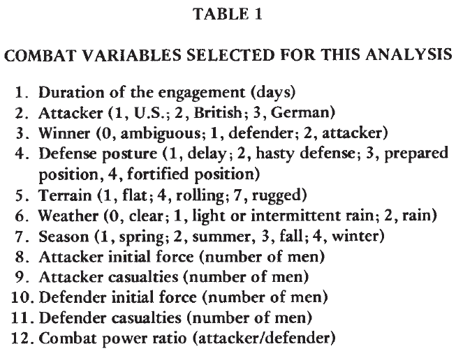
The general characteristics of the engagements are briefly described. Of the 60, there were 19 attacks by British forces, 28 by U.S. forces, and 13 by German forces. The attacker was successful in 34 cases; the defender, in 23; and the outcomes of 3 were ambiguous. With respect to terrain, 19 engagements occurred in flat terrain; 24 in rolling, or intermediate, terrain; and 17 in rugged, or difficult, terrain. Clear weather prevailed in 40 cases; 13 engagements were fought in light or intermittent rain; and 7 in medium or heavy rain. There were 28 spring and summer engagements and 32 fall and winter engagements.

Comparison of World War II Engagements With Historical Battles

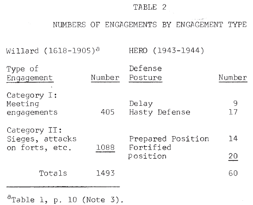
Since one purpose of this work is to repeat, in part, Willard’s analysis, comparison of these World War II engagements with the historical battles (1618-1905) studied by him will be useful. Table 2 shows a comparison of the distribution of battles by type. Willard’s cases were divided into two categories: I. meeting engagements, and II. sieges, attacks on forts, and similar operations. HERO’s World War II engagements were divided into four types based on the posture of the defender: 1. delay, 2. hasty defense, 3. prepared position, and 4. fortified position. If postures 1 and 2 are considered very roughly equivalent to Willard’s category I, then in both data sets the division into the two gross categories is approximately even.

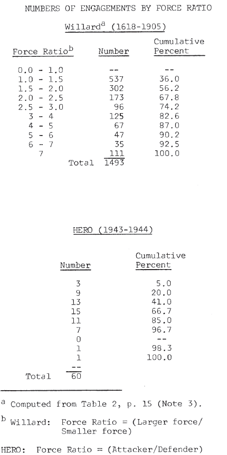
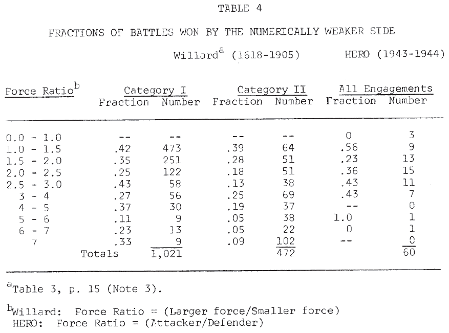
The distribution of engagements across force ratios, given in Table 3, indicated some differences. Willard’s engagements tend to cluster at the lower end of the scale (1-2) and at the higher end (4 and above), while the majority of the World War II engagements were found in mid-range (1.5 – 4) (Note 8). The frequency with which the numerically inferior force achieved victory is shown in Table 4. It is seen that in neither data set are force ratios good predictors of success in battle (Note 9).

Table 3.

Results of the Analysis Willard’s Correlation Analysis

There are two forms of the Lanchester equations. One represents the case in which firing units on both sides know the locations of their opponents and can shift their fire to a new target when a “kill” is achieved. This leads to the “square” law where the loss rate is proportional to the opponent’s size. The second form represents that situation in which only the general location of the opponent is known. This leads to the “linear” law in which the loss rate is proportional to the product of both force sizes.

As Willard points out, large battles are made up of many smaller fights. Some of these obey one law while others obey the other, so that the overall result should be a combination of the two. Starting with a general formulation of Lanchester’s equations, where g is the exponent of the target unit’s size (that is, g is 0 for the square law and 1 for the linear law), he derives the following linear equation:

log (nc/mc) = log E + g log (mo/no) (1)

where nc and mc are the casualties, E is related to the exchange ratio, and mo and no are the initial force sizes. Linear regression produces a value for g. However, instead of lying between 0 and 1, as expected, the) g‘s range from -.27 to -.87, with the majority lying around -.5. (Willard obtains several values for g by dividing his data base in various ways—by force ratio, by casualty ratio, by historical period, and so forth.) A negative g value is unpleasant. As Willard notes:

Military theorists should be disconcerted to find g < 0, for in this range the results seem to imply that if the Lanchester formulation is valid, the casualty-producing power of troops increases as they suffer casualties (Note 3).

From his results, Willard concludes that his analysis does not justify the use of Lanchester equations in large-scale situations (Note 10).

Analysis of the World War II Engagements

Willard’s computations were repeated for the HERO data set. For these engagements, regression produced a value of -.594 for g (Note 11), in striking agreement with Willard’s results. Following his reasoning would lead to the conclusion that either the Lanchester equations do not represent these engagements, or that the casualty producing power of forces increases as their size decreases.

However, since the Lanchester equations are so convenient analytically and their use is so widespread, it appeared worthwhile to reconsider this conclusion. In deriving equation (1), Willard used binomial expansions in which he retained only the leading terms. It seemed possible that the poor results might he due, in part, to this approximation. If the first two terms of these expansions are retained, the following equation results:

log (nc/mc) = log E + log (Mo-mc)/(no-nc) (2)

Repeating this regression on the basis of this equation leads to g = -.413 (Note 12), hardly an improvement over the initial results.

A second attempt was made to salvage this approach. Starting with raw OLI scores (Note 7), HERO analysts have computed “combat potentials” for both sides in these engagements, taking into account the operational factors of posture, vulnerability, and mobility; environmental factors like weather, season, and terrain; and (when the record warrants) psychological factors like troop training, morale, and the quality of leadership. Replacing the factor (mo/no) in Equation (1) by the combat power ratio produces the result) g = .466 (Note 13).

While this is an apparent improvement in the value of g, it is achieved at the expense of somewhat distorting the Lanchester concept. It does preserve the functional form of the equations, but it requires a somewhat strange definition of “killing rates.”

Analysis Based on the Differential Lanchester Equations

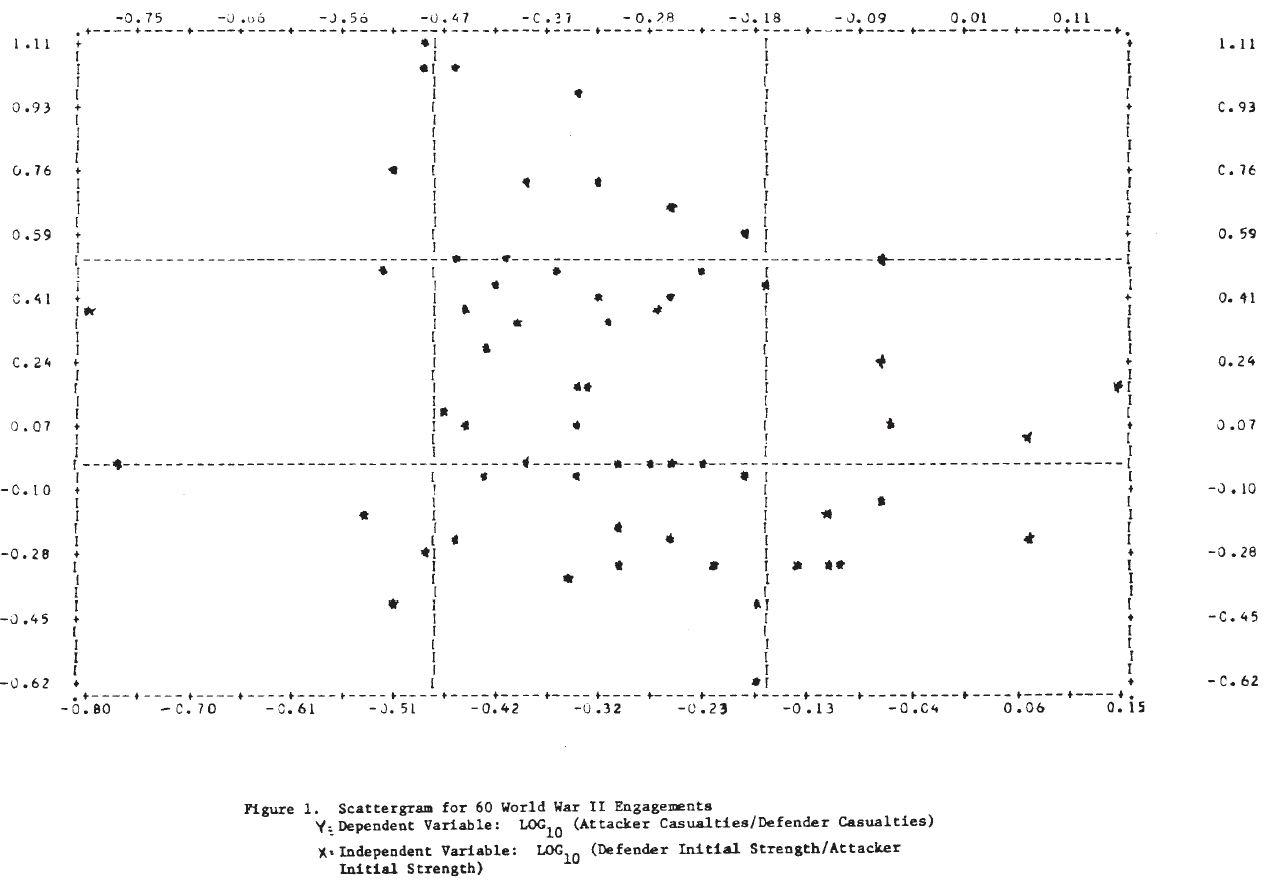
Analysis of the type carried out by Willard appears to produce very poor results for these World War II engagements. Part of the reason for this is apparent from Figure 1, which shows the scatterplot of the dependent variable, log (nc/mc), against the independent variable, log (mo/no). It is clear that no straight line will fit these data very well, and one with a positive slope would not be much worse than the “best” line found by regression. To expect the exponent to account for the wide variation in these data seems unreasonable.

Here, a simpler approach will be taken. Rather than use the data to attempt to discriminate directly between the square and the linear laws, they will be used to estimate linear coefficients under each assumption in turn, starting with the differential formulation rather than the integrated equations used by Willard.

In their simplest differential form, the Lanchester equations may be written;

Square Law; dA/dt = -kdD and dD/dt = kaA (3)

Linear law: dA/dt = -k’dAD and dD/dt = k’aAD (4)

where

A(D) is the size of the attacker (defender)

dA/dt (dD/dt) is the attacker’s (defender’s) loss rate,

ka, k’a (kd, k’d) are the attacker’s (defender’s) killing rates

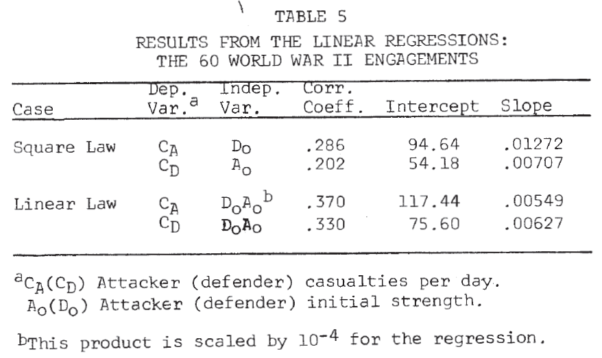
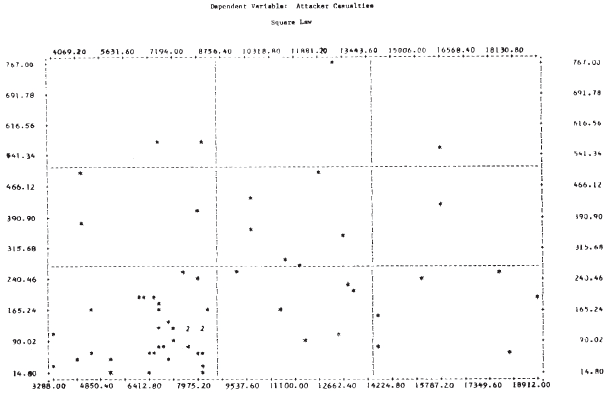
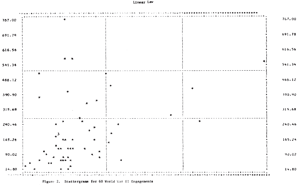
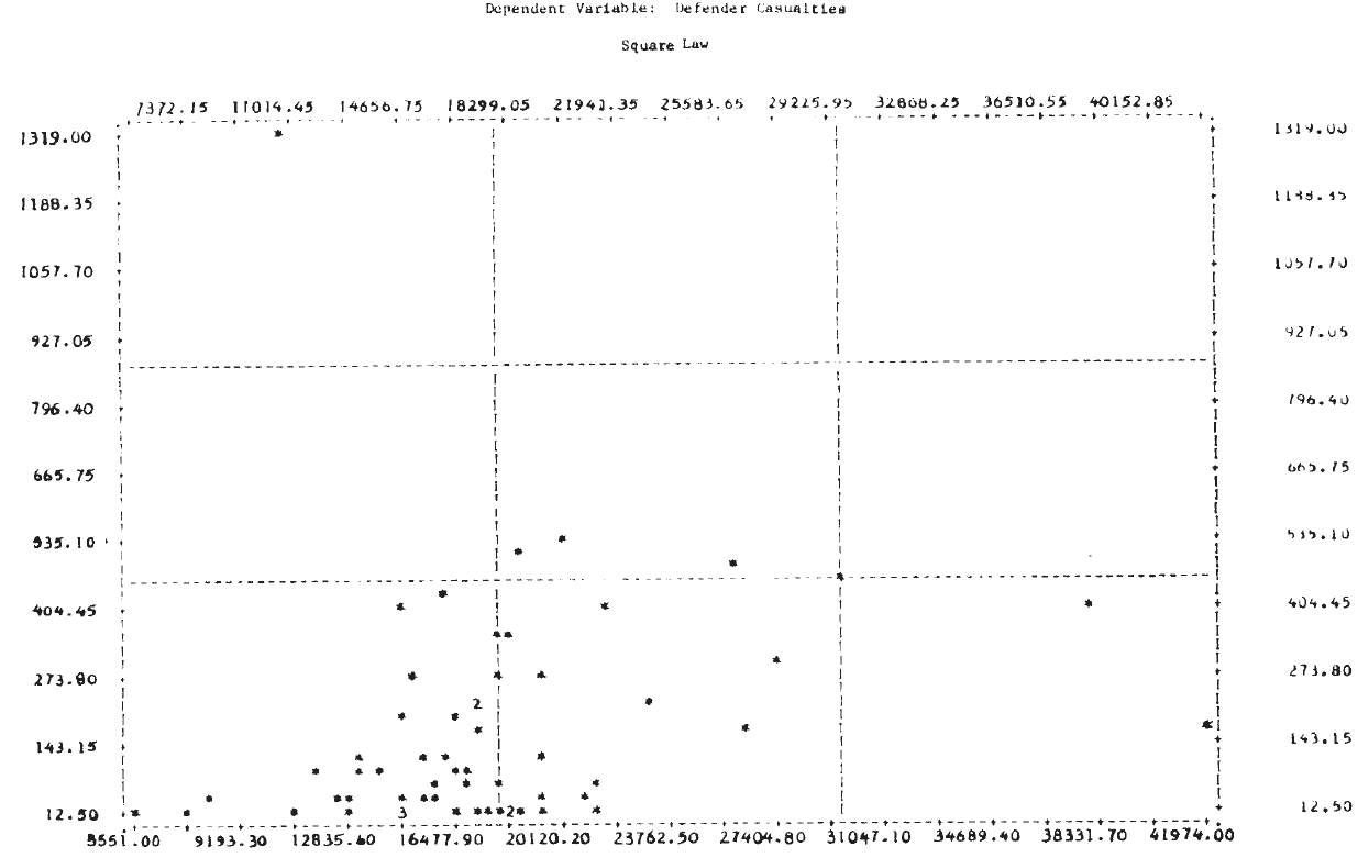
For this analysis, the day is taken as the basic time unit, and the loss rate per day is approximated by the casualties per day. Results of the linear regressions are given in Table 5. No conclusions should be drawn from the fact that the correlation coefficients are higher in the linear law case since this is expected for purely technical reasons (Note 14). A better picture of the relationships is again provided by the scatterplots in Figure 2. It is clear from these plots that, as in the case of the logarithmic forms, a single straight line will not fit the entire set of 60 engagements for either of the dependent variables.

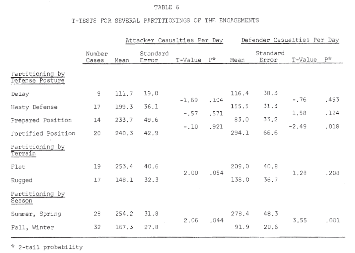
To investigate ways in which the data set might profitably be subdivided for analysis, T-tests of the means of the dependent variable were made for several partitionings of the data set. The results, shown in Table 6, suggest that dividing the engagements by defense posture might prove worthwhile.

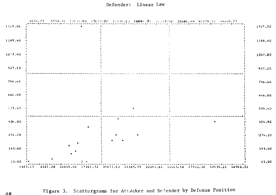
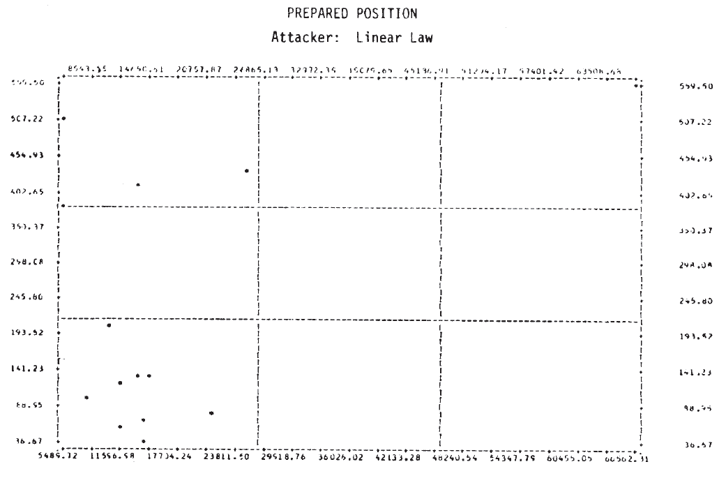
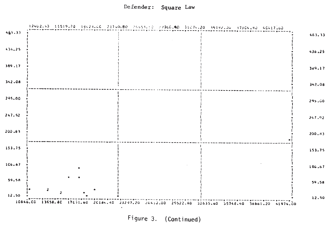
Results of the linear regressions by defense posture are shown in Table 7. For each posture, the equation that seemed to give a better fit to the data is underlined (Note 15). From this table, the following very tentative conclusions might be drawn:

  • In an attack on a fortified position, the attacker suffers casualties by the square law; the defender suffers casualties by the linear law. That is, the defender is aware of the attacker’s position, while the attacker knows only the general location of the defender. (This is similar to Deitchman’s guerrilla model. Note 16).
  • This situation is apparently reversed in the cases of attacks on prepared positions and hasty defenses.
  • Delaying situations seem to be treated better by the square law for both attacker and defender.

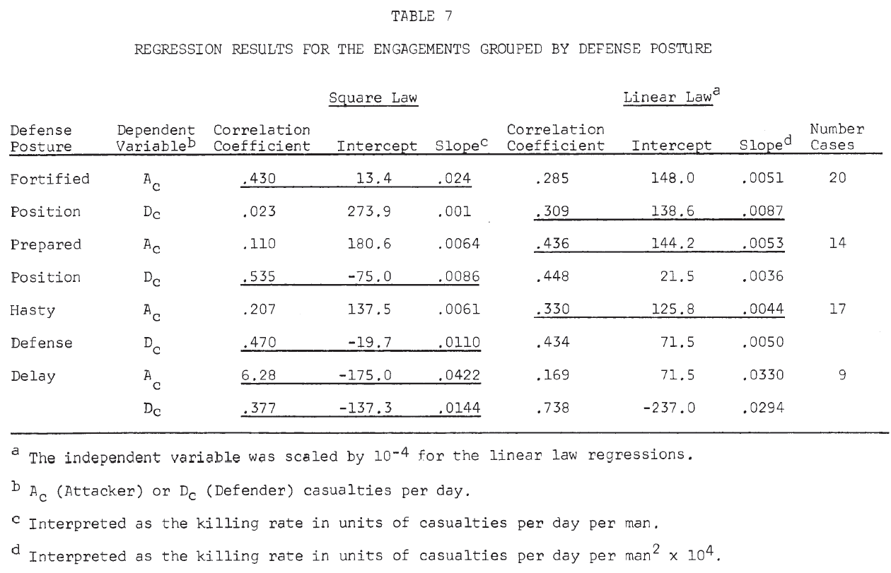
Table 8 summarizes the killing rates by defense posture. The defender has a much higher killing rate than the attacker (almost 3 to 1) in a fortified position. In a prepared position and hasty defense, the attacker appears to have the advantage. However, in a delaying action, the defender’s killing rate is again greater than the attacker’s (Note 17).

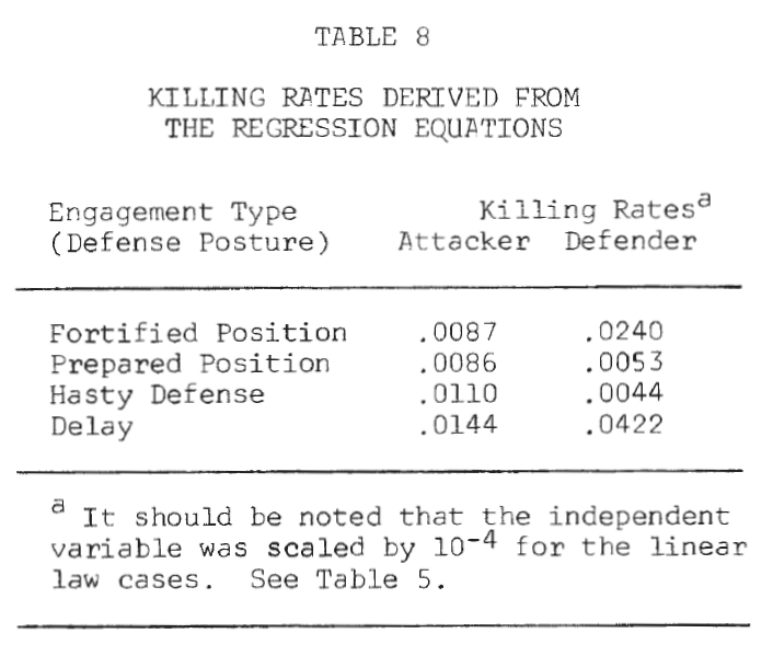
Figure 3 shows the scatterplots for these cases. Examination of these plots suggests that a tentative answer to the study question posed above might be: “Yes, casualties do appear to be related to the force sizes, but the relationship may not be a simple linear one.”

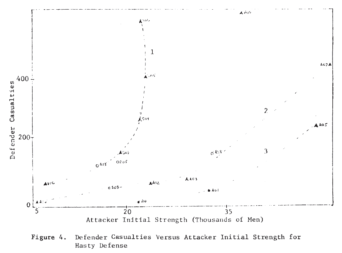
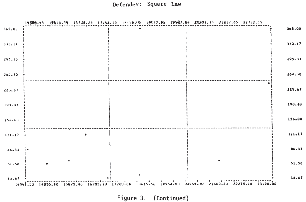
In several of these plots it appears that two or more functional forms may be involved. Consider, for example, the defender‘s casualties as a function of the attacker’s initial strength in the case of a hasty defense. This plot is repeated in Figure 4, where the points appear to fit the curves sketched there. It would appear that there are at least two, possibly three, separate relationships. Also on that plot, the individual engagements have been identified, and it is interesting to note that on the curve marked (1), five of the seven attacks were made by Germans—four of them from the Salerno campaign. It would appear from this that German attacks are associated with higher than average defender casualties for the attacking force size. Since there are so few data points, this cannot be more than a hint or interesting suggestion.

Future Research

This work suggests two conclusions that might have an impact on future lines of research on combat dynamics:

  • Tactics appear to be an important determinant of combat results. This conclusion, in itself, does not appear startling, at least not to the military. However, it does not always seem to have been the case that tactical questions have been considered seriously by analysts in their studies of the effects of varying force levels and force mixes.
  • Historical data of this type offer rich opportunities for studying the effects of tactics. For example, consideration of the narrative accounts of these battles might permit re-coding the engagements into a larger, more sensitive set of engagement categories. (It would, of course, then be highly desirable to add more engagements to the data set.)

While predictions of the future are always dangerous, I would nevertheless like to suggest what appears to be a possible trend. While military analysis of the past two decades has focused almost exclusively on the hardware of weapons systems, at least part of our future analysis will be devoted to the more behavioral aspects of combat.

Janice Bloom Fain, a Senior Associate of CACI, lnc., is a physicist whose special interests are in the applications of computer simulation techniques to industrial and military operations; she is the author of numerous reports and articles in this field. This paper was presented by Dr. Fain at the Military Operations Research Symposium at Fort Eustis, Virginia.

NOTES

[1.] J. H. Engel, “A Verification of Lanchester’s Law,” Operations Research 2, 163-171 (1954).

[2.] For example, see R. L. Helmbold, “Some Observations on the Use of Lanchester’s Theory for Prediction,” Operations Research 12, 778-781 (1964); H. K. Weiss, “Lanchester-Type Models of Warfare,” Proceedings of the First International Conference on Operational Research, 82-98, ORSA (1957); H. K. Weiss, “Combat Models and Historical Data; The U.S. Civil War,” Operations Research 14, 750-790 (1966).

[3.] D. Willard, “Lanchester as a Force in History: An Analysis of Land Battles of the Years 1618-1905,” RAC-TD-74, Research Analysis Corporation (1962). what appears to be a possible trend. While military analysis of the past two decades has focused almost exclusively on the hardware of weapons systems, at least part of our future analysis will be devoted to the more behavioral aspects of combat.

[4.] The method of computing the killing rates forced a fit at the beginning and end of the battles. See W. Fain, J. B. Fain, L. Feldman, and S. Simon, “Validation of Combat Models Against Historical Data,” Professional Paper No. 27, Center for Naval Analyses, Arlington, Virginia (1970).

[5.] HERO, “A Study of the Relationship of Tactical Air Support Operations to Land Combat, Appendix B, Historical Data Base.” Historical Evaluation and Research Organization, report prepared for the Defense Operational Analysis Establishment, U.K.T.S.D., Contract D-4052 (1971).

[6.] T. N. Dupuy, The Quantified Judgment Method of Analysis of Historical Combat Data, HERO Monograph, (January 1973); HERO, “Statistical Inference in Analysis in Combat,” Annex F, Historical Data Research on Tactical Air Operations, prepared for Headquarters USAF, Assistant Chief of Staff for Studies and Analysis, Contract No. F-44620-70-C-0058 (1972).

[7.] The Operational Lethality Index (OLI) is a measure of weapon effectiveness developed by HERO.

[8.] Since Willard’s data did not indicate which side was the attacker, his force ratio is defined to be (larger force/smaller force). The HERO force ratio is (attacker/defender).

[9.] Since the criteria for success may have been rather different for the two sets of battles, this comparison may not be very meaningful.

[10.] This work includes more complex analysis in which the possibility that the two forces may be engaging in different types of combat is considered, leading to the use of two exponents rather than the single one, Stochastic combat processes are also treated.

[11.] Correlation coefficient = -.262;

Intercept = .00115; slope = -.594.

[12.] Correlation coefficient = -.184;

Intercept = .0539; slope = -,413.

[13.] Correlation coefficient = .303;

Intercept = -.638; slope = .466.

[14.] Correlation coefficients for the linear law are inflated with respect to the square law since the independent variable is a product of force sizes and, thus, has a higher variance than the single force size unit in the square law case.

[15.] This is a subjective judgment based on the following considerations Since the correlation coefficient is inflated for the linear law, when it is lower the square law case is chosen. When the linear law correlation coefficient is higher, the case with the intercept closer to 0 is chosen.

[16.] S. J. Deitchman, “A Lanchester Model of Guerrilla Warfare,” Operations Research 10, 818-812 (1962).

[17.] As pointed out by Mr. Alan Washburn, who prepared a critique on this paper, when comparing numerical values of the square law and linear law killing rates, the differences in units must be considered. (See footnotes to Table 7).

What Is A Breakpoint?

French retreat from Russia in 1812 by Illarion Mikhailovich Pryanishnikov (1812) [Wikipedia]

After discussing with Chris the series of recent posts on the subject of breakpoints, it seemed appropriate to provide a better definition of exactly what a breakpoint is.

Dorothy Kneeland Clark was the first to define the notion of a breakpoint in her study, Casualties as a Measure of the Loss of Combat Effectiveness of an Infantry Battalion (Operations Research Office, The Johns Hopkins University: Baltimore, 1954). She found it was not quite as clear-cut as it seemed and the working definition she arrived at was based on discussions and the specific combat outcomes she found in her data set [pp 9-12].

DETERMINATION OF BREAKPOINT

The following definitions were developed out of many discussions. A unit is considered to have lost its combat effectiveness when it is unable to carry out its mission. The onset of this inability constitutes a breakpoint. A unit’s mission is the objective assigned in the current operations order or any other instructional directive, written or verbal. The objective may be, for example, to attack in order to take certain positions, or to defend certain positions. 

How does one determine when a unit is unable to carry out its mission? The obvious indication is a change in operational directive: the unit is ordered to stop short of its original goal, to hold instead of attack, to withdraw instead of hold. But one or more extraneous elements may cause the issue of such orders: 

(1) Some other unit taking part in the operation may have lost its combat effectiveness, and its predicament may force changes, in the tactical plan. For example the inability of one infantry battalion to take a hill may require that the two adjoining battalions be stopped to prevent exposing their flanks by advancing beyond it. 

(2) A unit may have been assigned an objective on the basis of a G-2 estimate of enemy weakness which, as the action proceeds, proves to have been over-optimistic. The operations plan may, therefore, be revised before the unit has carried out its orders to the point of losing combat effectiveness. 

(3) The commanding officer, for reasons quite apart from the tactical attrition, may change his operations plan. For instance, General Ridgway in May 1951 was obliged to cancel his plans for a major offensive north of the 38th parallel in Korea in obedience to top level orders dictated by political considerations. 

(4) Even if the supposed combat effectiveness of the unit is the determining factor in the issuance of a revised operations order, a serious difficulty in evaluating the situation remains. The commanding officer’s decision is necessarily made on the basis of information available to him plus his estimate of his unit’s capacities. Either or both of these bases may be faulty. The order may belatedly recognize a collapse which has in factor occurred hours earlier, or a commanding officer may withdraw a unit which could hold for a much longer time. 

It was usually not hard to discover when changes in orders resulted from conditions such as the first three listed above, but it proved extremely difficult to distinguish between revised orders based on a correct appraisal of the unit’s combat effectiveness and those issued in error. It was concluded that the formal order for a change in mission cannot be taken as a definitive indication of the breakpoint of a unit. It seemed necessary to go one step farther and search the records to learn what a given battalion did regardless of provisions in formal orders… 

CATEGORIES OF BREAKPOINTS SELECTED 

In the engagements studied the following categories of breakpoint were finally selected: 

Category of Breakpoint 

No. Analyzed 

I. Attack [Symbol] rapid reorganization [Symbol] attack 

9 

II. Attack [Symbol] defense (no longer able to attack without a few days of recuperation and reinforcement 

21 

III. Defense [Symbol] withdrawal by order to a secondary line 

13 

IV. Defense [Symbol] collapse 

5 

Disorganization and panic were taken as unquestionable evidence of loss of combat effectiveness. It appeared, however, that there were distinct degrees of magnitude in these experiences. In addition to the expected breakpoints at attack [Symbol] defense and defense [Symbol] collapse, a further category, I, seemed to be indicated to include situations in which an attacking battalion was ‘pinned down” or forced to withdraw in partial disorder but was able to reorganize in 4 to 24 hours and continue attacking successfully. 

Category II includes (a) situations in which an attacking battalion was ordered into the defensive after severe fighting or temporary panic; (b) situations in which a battalion, after attacking successfully, failed to gain ground although still attempting to advance and was finally ordered into defense, the breakpoint being taken as occurring at the end of successful advance. In other words, the evident inability of the unit to fulfill its mission was used as the criterion for the breakpoint whether orders did or did not recognize its inability. Battalions after experiencing such a breakpoint might be able to recuperate in a few days to the point of renewing successful attack or might be able to continue for some time in defense. 

The sample of breakpoints coming under category IV, defense [Symbol] collapse, proved to be very small (5) and unduly weighted in that four of the examples came from the same engagement. It was, therefore, discarded as probably not representative of the universe of category IV breakpoints,* and another category (III) was added: situations in which battalions on the defense were ordered withdrawn to a quieter sector. Because only those instances were included in which the withdrawal orders appeared to have been dictated by the condition of the unit itself, it is believed that casualty levels for this category can be regarded as but slightly lower than those associated with defense [Symbol] collapse. 

In both categories II and III, “‘defense” represents an active situation in which the enemy is attacking aggressively. 

* It had been expected that breakpoints in this category would be associated with very high losses. Such did not prove to be the case. In whatever way the data were approached, most of the casualty averages were only slightly higher than those associated with category II (attack [Symbol] defense), although the spread in data was wider. It is believed that factors other than casualties, such as bad weather, difficult terrain, and heavy enemy artillery fire undoubtedly played major roles in bringing about the collapse in the four units taking part in the same engagement. Furthermore, the casualty figures for the four units themselves is in question because, as the situation deteriorated, many of the men developed severe cases of trench foot and combat exhaustion, but were not evacuated, as they would have been in a less desperate situation, and did not appear in the casualty records until they had made their way to the rear after their units had collapsed.

In 1987-1988, Trevor Dupuy and colleagues at Data Memory Systems, Inc. (DMSi), Janice Fain, Rich Anderson, Gay Hammerman, and Chuck Hawkins sought to create a broader, more generally applicable definition for breakpoints for the study, Forced Changes of Combat Posture (DMSi, Fairfax, VA, 1988) [pp. I-2-3]

The combat posture of a military force is the immediate intention of its commander and troops toward the opposing enemy force, together with the preparations and deployment to carry out that intention. The chief combat postures are attack, defend, delay, and withdraw.

A change in combat posture (or posture change) is a shift from one posture to another, as, for example, from defend to attack or defend to withdraw. A posture change can be either voluntary or forced. 

A forced posture change (FPC) is a change in combat posture by a military unit that is brought about, directly or indirectly, by enemy action. Forced posture changes are characteristically and almost always changes to a less aggressive posture. The most usual FPCs are from attack to defend and from defend to withdraw (or retrograde movement). A change from withdraw to combat ineffectiveness is also possible. 

Breakpoint is a term sometimes used as synonymous with forced posture change, and sometimes used to mean the collapse of a unit into ineffectiveness or rout. The latter meaning is probably more common in general usage, while forced posture change is the more precise term for the subject of this study. However, for brevity and convenience, and because this study has been known informally since its inception as the “Breakpoints” study, the term breakpoint is sometimes used in this report. When it is used, it is synonymous with forced posture change.

Hopefully this will help clarify the previous discussions of breakpoints on the blog.

Response 3 (Breakpoints)

This is in response to long comment by Clinton Reilly about Breakpoints (Forced Changes in Posture) on this thread:

Breakpoints in U.S. Army Doctrine

Reilly starts with a very nice statement of the issue:

Clearly breakpoints are crucial when modelling battlefield combat. I have read extensively about it using mostly first hand accounts of battles rather than high level summaries. Some of the major factors causing it appear to be loss of leadership (e.g. Harald’s death at Hastings), loss of belief in the units capacity to achieve its objectives (e.g. the retreat of the Old Guard at Waterloo, surprise often figured in Mongol successes, over confidence resulting in impetuous attacks which fail dramatically (e.g. French attacks at Agincourt and Crecy), loss of control over the troops (again Crecy and Agincourt) are some of the main ones I can think of off hand.

The break-point crisis seems to occur against a background of confusion, disorder, mounting casualties, increasing fatigue and loss of morale. Casualties are part of the background but not usually the actual break point itself.

He then states:

Perhaps a way forward in the short term is to review a number of first hand battle accounts (I am sure you can think of many) and calculate the percentage of times these factors and others appear as breakpoints in the literature.

This has been done. In effect this is what Robert McQuie did in his article and what was the basis for the DMSI breakpoints study.

Battle Outcomes: Casualty Rates As a Measure of Defeat

Mr. Reilly then concludes:

Why wait for the military to do something? You will die of old age before that happens!

That is distinctly possible. If this really was a simple issue that one person working for a year could produce a nice definitive answer for…..it would have already been done !!!

Let us look at the 1988 Breakpoints study. There was some effort leading up to that point. Trevor Dupuy and DMSI had already looked into the issue. This included developing a database of engagements (the Land Warfare Data Base or LWDB) and using that to examine the nature of breakpoints. The McQuie article was developed from this database, and his article was closely coordinated with Trevor Dupuy. This was part of the effort that led to the U.S. Army’s Concepts Analysis Agency (CAA) to issue out a RFP (Request for Proposal). It was competitive. I wrote the proposal that won the contract award, but the contract was given to Dr. Janice Fain to lead. My proposal was more quantitative in approach than what she actually did. Her effort was more of an intellectual exploration of the issue. I gather this was done with the assumption that there would be a follow-on contract (there never was). Now, up until that point at least a man-year of effort had been expended, and if you count the time to develop the databases used, it was several man-years.

Now the Breakpoints study was headed up by Dr. Janice B. Fain, who worked on it for the better part of a year. Trevor N. Dupuy worked on it part-time. Gay M. Hammerman conducted the interview with the veterans. Richard C. Anderson researched and created an additional 24 engagements that had clear breakpoints in them for the study (that is DMSI report 117B). Charles F. Hawkins was involved in analyzing the engagements from the LWDB. There were several other people also involved to some extent. Also, 39 veterans were interviewed for this effort. Many were brought into the office to talk about their experiences (that was truly entertaining). There were also a half-dozen other staff members and consultants involved in the effort, including Lt. Col. James T. Price (USA, ret), Dr. David Segal (sociologist), Dr. Abraham Wolf (a research psychologist), Dr. Peter Shapiro (social psychology) and Col. John R. Brinkerhoff (USA, ret). There were consultant fees, travel costs and other expenses related to that. So, the entire effort took at least three “man-years” of effort. This was what was needed just get to the point where we are able to take the next step.

This is not something that a single scholar can do. That is why funding is needed.

As to dying of old age before that happens…..that may very well be the case. Right now, I am working on two books, one of them under contract. I sort of need to finish those up before I look at breakpoints again. After that, I will decide whether to work on a follow-on to America’s Modern Wars (called Future American Wars) or work on a follow-on to War by Numbers (called War by Numbers II…being the creative guy that I am). Of course, neither of these books are selling well….so perhaps my time would be better spent writing another Kursk book, or any number of other interesting projects on my plate. Anyhow, if I do War by Numbers II, then I do plan on investing several chapters into addressing breakpoints. This would include using the 1,000+ cases that now populate our combat databases to do some analysis. This is going to take some time. So…….I may get to it next year or the year after that, but I may not. If someone really needs the issue addressed, they really need to contract for it.

Breakpoints in U.S. Army Doctrine

U.S. Army prisoners of war captured by German forces during the Battle of the Bulge in 1944. [Wikipedia]

One of the least studied aspects of combat is battle termination. Why do units in combat stop attacking or defending? Shifts in combat posture (attack, defend, delay, withdrawal) are usually voluntary, directed by a commander, but they can also be involuntary, as a result of direct or indirect enemy action. Why do involuntary changes in combat posture, known as breakpoints, occur?

As Chris pointed out in a previous post, the topic of breakpoints has only been addressed by two known studies since 1954. Most existing military combat models and wargames address breakpoints in at least a cursory way, usually through some calculation based on personnel casualties. Both of the breakpoints studies suggest that involuntary changes in posture are seldom related to casualties alone, however.

Current U.S. Army doctrine addresses changes in combat posture through discussions of culmination points in the attack, and transitions from attack to defense, defense to counterattack, and defense to retrograde. But these all pertain to voluntary changes, not breakpoints.

Army doctrinal literature has little to say about breakpoints, either in the context of friendly forces or potential enemy combatants. The little it does say relates to the effects of fire on enemy forces and is based on personnel and material attrition.

According to ADRP 1-02 Terms and Military Symbols, an enemy combat unit is considered suppressed after suffering 3% personnel casualties or material losses, neutralized by 10% losses, and destroyed upon sustaining 30% losses. The sources and methodology for deriving these figures is unknown, although these specific terms and numbers have been a part of Army doctrine for decades.

The joint U.S. Army and U.S. Marine Corps vision of future land combat foresees battlefields that are highly lethal and demanding on human endurance. How will such a future operational environment affect combat performance? Past experience undoubtedly offers useful insights but there seems to be little interest in seeking out such knowledge.

Trevor Dupuy criticized the U.S. military in the 1980s for its lack of understanding of the phenomenon of suppression and other effects of fire on the battlefield, and its seeming disinterest in studying it. Not much appears to have changed since then.

C-WAM 4 (Breakpoints)

A breakpoint or involuntary change in posture is an essential part of modeling. There is a breakpoint methodology in C-WAM. According to slide 18 and rule book section 5.7.2 is that ground unit below 50% strength can only defend. It is removed at below 30% strength. I gather this is a breakpoint for a brigade.

C-WAM 2

Let me just quote from Chapter 18 (Modeling Warfare) of my book War by Numbers: Understanding Conventional Combat (pages 288-289):

The original breakpoints study was done in 1954 by Dorothy Clark of ORO [which can be found here].[1] It examined forty-three battalion-level engagements where the units “broke,” including measuring the percentage of losses at the time of the break. Clark correctly determined that casualties were probably not the primary cause of the breakpoint and also declared the need to look at more data. Obviously, forty-three cases of highly variable social science-type data with a large number of variables influencing them are not enough for any form of definitive study. Furthermore, she divided the breakpoints into three categories, resulting in one category based upon only nine observations. Also, as should have been obvious, this data would apply only to battalion-level combat. Clark concluded “The statement that a unit can be considered no longer combat effective when it has suffered a specific casualty percentage is a gross oversimplification not supported by combat data.” She also stated “Because of wide variations in data, average loss percentages alone have limited meaning.”[2]

Yet, even with her clear rejection of a percent loss formulation for breakpoints, the 20 to 40 percent casualty breakpoint figures remained in use by the training and combat modeling community. Charts in the 1964 Maneuver Control field manual showed a curve with the probability of unit break based on percentage of combat casualties.[3] Once a defending unit reached around 40 percent casualties, the chance of breaking approached 100 percent. Once an attacking unit reached around 20 percent casualties, the chance of it halting (type I break) approached 100% and the chance of it breaking (type II break) reached 40 percent. These data were for battalion-level combat. Because they were also applied to combat models, many models established a breakpoint of around 30 or 40 percent casualties for units of any size (and often applied to division-sized units).

To date, we have absolutely no idea where these rule-of-thumb formulations came from and despair of ever discovering their source. These formulations persist despite the fact that in fifteen (35%) of the cases in Clark’s study, the battalions had suffered more than 40 percent casualties before they broke. Furthermore, at the division-level in World War II, only two U.S. Army divisions (and there were ninety-one committed to combat) ever suffered more than 30% casualties in a week![4] Yet, there were many forced changes in combat posture by these divisions well below that casualty threshold.

The next breakpoints study occurred in 1988.[5] There was absolutely nothing of any significance (meaning providing any form of quantitative measurement) in the intervening thirty-five years, yet there were dozens of models in use that offered a breakpoint methodology. The 1988 study was inconclusive, and since then nothing further has been done.[6]

This seemingly extreme case is a fairly typical example. A specific combat phenomenon was studied only twice in the last fifty years, both times with inconclusive results, yet this phenomenon is incorporated in most combat models. Sadly, similar examples can be pulled for virtually each and every phenomena of combat being modeled. This failure to adequately examine basic combat phenomena is a problem independent of actual combat modeling methodology.

Footnotes:

[1] Dorothy K. Clark, Casualties as a Measure of the Loss of Combat Effectiveness of an Infantry Battalion (Operations Research Office, Johns Hopkins University, 1954).

 [2] Ibid, page 34.

[3] Headquarters, Department of the Army, FM 105-5 Maneuver Control (Washington, D.C., December, 1967), pages 128-133.

[4] The two exceptions included the U.S. 106th Infantry Division in December 1944, which incidentally continued fighting in the days after suffering more than 40 percent losses, and the Philippine Division upon its surrender in Bataan on 9 April 1942 suffered 100% losses in one day in addition to very heavy losses in the days leading up to its surrender.

[5] This was HERO Report number 117, Forced Changes of Combat Posture (Breakpoints) (Historical Evaluation and Research Organization, Fairfax, VA., 1988). The intervening years between 1954 and 1988 were not entirely quiet. See HERO Report number 112, Defeat Criteria Seminar, Seminar Papers on the Evaluation of the Criteria for Defeat in Battle (Historical Evaluation and Research Organization, Fairfax, VA., 12 June 1987) and the significant article by Robert McQuie, “Battle Outcomes: Casualty Rates as a Measure of Defeat” in Army, issue 37 (November 1987). Some of the results of the 1988 study was summarized in the book by Trevor N. Dupuy, Understanding Defeat: How to Recover from Loss in Battle to Gain Victory in War (Paragon House Publishers, New York, 1990).

 [6] The 1988 study was the basis for Trevor Dupuy’s book: Col. T. N. Dupuy, Understanding Defeat: How to Recover From Loss in Battle to Gain Victory in War (Paragon House Publishers, New York, 1990).

Also see:

Battle Outcomes: Casualty Rates As a Measure of Defeat

[NOTE: Post updated to include link to Dorothy Clark’s original breakpoints study.]

Abstraction and Aggregation in Wargame Modeling

[IPMS/USA Reviews]

“All models are wrong, some models are useful.” – George Box

Models, no matter what their subjects, must always be an imperfect copy of the original. The term “model” inherently has this connotation. If the subject is exact and precise, then it is a duplicate, a replica, a clone, or a copy, but not a “model.” The most common dimension to be compromised is generally size, or more literally the three spatial dimensions of length, width and height. A good example of this would be a scale model airplane, generally available in several ratios from the original, such as 1/144, 1/72 or 1/48 (which are interestingly all factors of 12 … there are also 1/100 for the more decimal-minded). These mean that the model airplane at 1/72 scale would be 72 times smaller … take the length, width and height measurements of the real item, and divide by 72 to get the model’s value.

If we take the real item’s weight and divide by 72, we would not expect our model to weight 72 times less! Not unless the same or similar materials would be used, certainly. Generally, the model has a different purpose than replicating the subject’s functionality. It is helping to model the subject’s qualities, or to mimic them in some useful way. In the case of the 1/72 plastic model airplane of the F-15J fighter, this might be replicating the sight of a real F-15J, to satisfy the desire of the youth to look at the F-15J and to imagine themselves taking flight. Or it might be for pilots at a flight school to mimic air combat with models instead of ha

The model aircraft is a simple physical object; once built, it does not change over time (unless you want to count dropping it and breaking it…). A real F-15J, however, is a dynamic physical object, which changes considerably over the course of its normal operation. It is loaded with fuel, ordnance, both of which have a huge effect on its weight, and thus its performance characteristics. Also, it may be occupied by different crew members, whose experience and skills may vary considerably. These qualities of the unit need to be taken into account, if the purpose of the model is to represent the aircraft. The classic example of this is a flight envelope model of an F-15A/C:

[Quora]

This flight envelope itself is a model, it represents the flight characteristics of the F-15 using two primary quantitative axes – altitude and speed (in numbers of mach), and also throttle setting. Perhaps the most interesting thing about this is the realization than an F-15 slows down as it descends. Are these particular qualities of an F-15 required to model air combat involving such and aircraft?

How to Apply This Modeling Process to a Wargame?

The purpose of the war game is to model or represent the possible outcome of a real combat situation, played forward in the model at whatever pace and scale the designer has intended.

As mentioned previously, my colleague and I are playing Asian Fleet, a war game that covers several types of naval combat, including those involving air units, surface units and submarine units. This was published in 2007, and updated in 2010. We’ve selected a scenario that has only air units on either side. The premise of this scenario is quite simple:

The Chinese air force, in trying to prevent the United States from intervening in a Taiwan invasion, will carry out an attack on the SDF as well as the US military base on Okinawa. Forces around Shanghai consisting of state-of-the-art fighter bombers and long-range attack aircraft have been placed for the invasion of Taiwan, and an attack on Okinawa would be carried out with a portion of these forces. [Asian Fleet Scenario Book]

Of course, this game is a model of reality. The infinite geospatial and temporal possibilities of space-time which is so familiar to us has been replaced by highly aggregated discreet buckets, such as turns that may last for a day, or eight hours. Latitude, longitude and altitude are replaced with a two-dimensional hexagonal “honey comb” surface. Hence, distance is no longer computed in miles or meters, but rather in “hexes”, each of which is about 50 nautical miles. Aircraft are effectively aloft, or on the ground, although a “high mission profile” will provide endurance benefits. Submarines are considered underwater, or may use “deep mode” attempting to hide from sonar searches.

Maneuver units are represented by “counters” or virtual chits to be moved about the map as play progresses. Their level of aggregation varies from large and powerful ships and subs represented individually, to smaller surface units and weaker subs grouped and represented by a single counter (a “flotilla”), to squadrons or regiments of aircraft represented by a single counter. Depending upon the nation and the military branch, this may be a few as 3-5 aircraft in a maritime patrol aircraft (MPA) detachment (“recon” in this game), to roughly 10-12 aircraft in a bomber unit, to 24 or even 72 aircraft in a fighter unit (“interceptor” in this game).

Enough Theory, What Happened?!

The Chinese Air Force mobilized their H6H bomber, escorted by large numbers of Flankers (J11 and Su-30MK2 fighters from the Shanghai area, and headed East towards Okinawa. The US Air Force F-15Cs supported by airborne warning and control system (AWACS) detected this inbound force and delayed engagement until their Japanese F-15J unit on combat air patrol (CAP) could support them, and then engaged the Chinese force about 50 miles from the AWACS orbits. In this game, air combat is broken down into two phases, long-range air to air (LRAA) combat (aka beyond visual range, BVR), and “regular” air combat, or within visual range (WVR) combat.

In BVR combat, only units marked as equipped with BVR capability may attack:

  • 2 x F-15C units have a factor of 32; scoring a hit in 5 out of 10 cases, or roughly 50%.
  • Su-30MK2 unit has a factor of 16; scoring a hit in 4 out of 10 cases, ~40%.

To these numbers a modifier of +2 exists when the attacker is supported by AWACS, so the odds to score a hit increase to roughly 70% for the F-15Cs … but in our example they miss, and the Chinese shot misses as well. Thus, the combat proceeds to WVR.

In WVR combat, each opposing side sums their aerial combat factors:

  • 2 x F-15C (32) + F-15J (13) = 45
  • Su-30MK2 (15) + J11 (13) + H6H (1) = 29

These two numbers are then expressed as a ratio, attacker-to-defender (45:29), and rounded down in favor of the defender (1:1), and then a ten-sided-die (d10) is rolled to consult the Air-to-Air Combat Results Table, on the “CAP/AWACS Interception” line. The die was rolled, and a result of “0/0r” was achieved, which basically says that neither side takes losses, but the defender is turned back from the mission (“r” being code for “return to base”). Given the +2 modifier for the AWACS, the worst outcome for the Allies would be a mutual return to base result (“0r/0r”). The best outcome would be inflicting two “steps” of damage, and sending the rest home (“0/2r”). A step of loss is about one half of an air unit, represented by flipping over the counter or chit, and operating with the combat factors at about half strength.

To sum this up, as the Allied commander, my conclusion was that the Americans were hung-over or asleep for this engagement.

I am encouraged by some similarities between this game and the fantastic detail that TDI has just posted about the DACM model, here and here. Thus, I plan to not only dissect this Asian Fleet game (VGAF), but also go a gap analysis between VGAF and DACM.

The Dupuy Air Campaign Model (DACM)

[The article below is reprinted from the April 1997 edition of The International TNDM Newsletter. A description of the TDI Air Model Historical Data Study can be found here.]

The Dupuy Air Campaign Model
by Col. Joseph A. Bulger, Jr., USAF, Ret.

The Dupuy Institute, as part of the DACM [Dupuy Air Campaign Model], created a draft model in a spreadsheet format to show how such a model would calculate attrition. Below are the actual printouts of the “interim methodology demonstration,” which shows the types of inputs, outputs, and equations used for the DACM. The spreadsheet was created by Col. Bulger, while many of the formulae were the work of Robert Shaw.

Response 2 (Performance of Armies)

In an exchange with one of readers, he mentioned that about the possibility to quantifiably access the performances of armies and produce a ranking from best to worst. The exchange is here:

The Dupuy Institute Air Model Historical Data Study

We have done some work on this, and are the people who have done the most extensive published work on this. Swedish researcher Niklas Zetterling in his book Normandy 1944: German Military Organization, Combat Power and Organizational Effectiveness also addresses this subject, as he has elsewhere, for example, an article in The International TNDM Newsletter, volume I, No. 6, pages 21-23 called “CEV Calculations in Italy, 1943.” It is here: http://www.dupuyinstitute.org/tdipub4.htm

When it came to measuring the differences in performance of armies, Martin van Creveld referenced Trevor Dupuy in his book Fighting Power: German and U.S. Army Performance, 1939-1945, pages 4-8.

What Trevor Dupuy has done is compare the performances of both overall forces and individual divisions based upon his Quantified Judgment Model (QJM). This was done in his book Numbers, Predictions and War: The Use of History to Evaluate and Predict the Outcome of Armed Conflict. I bring the readers attention to pages ix, 62-63, Chapter 7: Behavioral Variables in World War II (pages 95-110), Chapter 9: Reliably Representing the Arab-Israeli Wars (pages 118-139), and in particular page 135, and pages 163-165. It was also discussed in Understanding War: History and Theory of Combat, Chapter Ten: Relative Combat Effectiveness (pages 105-123).

I ended up dedicating four chapters in my book War by Numbers: Understanding Conventional Combat to the same issue. One of the problems with Trevor Dupuy’s approach is that you had to accept his combat model as a valid measurement of unit performance. This was a reach for many people, especially those who did not like his conclusions to start with. I choose to simply use the combined statistical comparisons of dozens of division-level engagements, which I think makes the case fairly convincingly without adding a construct to manipulate the data. If someone has a disagreement with my statistical compilations and the results and conclusions from it, I have yet to hear them. I would recommend looking at Chapter 4: Human Factors (pages 16-18), Chapter 5: Measuring Human Factors in Combat: Italy 1943-1944 (pages 19-31), Chapter 6: Measuring Human Factors in Combat: Ardennes and Kursk (pages 32-48), and Chapter 7: Measuring Human Factors in Combat: Modern Wars (pages 49-59).

Now, I did end up discussing Trevor Dupuy’s model in Chapter 19: Validation of the TNDM and showing the results of the historical validations we have done of his model, but the model was not otherwise used in any of the analysis done in the book.

But….what we (Dupuy and I) have done is a comparison between forces that opposed each other. It is a measurement of combat value relative to each other. It is not an absolute measurement that can be compared to other armies in different times and places. Trevor Dupuy toyed with this on page 165 of NPW, but this could only be done by assuming that combat effectiveness of the U.S. Army in WWII was the same as the Israeli Army in 1973.

Anyhow, it is probably impossible to come up with a valid performance measurement that would allow you to rank an army from best to worse. It is possible to come up with a comparative performance measurement of armies that have faced each other. This, I believe we have done, using different methodologies and different historical databases. I do believe it would be possible to then determine what the different factors are that make up this difference. I do believe it would be possible to assign values or weights to those factors. I believe this would be very useful to know, in light of the potential training and organizational value of this knowledge.

The Dupuy Institute Air Model Historical Data Study

British Air Ministry aerial combat diagram that sought to explain how the RAF had fought off the Luftwaffe. [World War II Today]

[The article below is reprinted from the April 1997 edition of The International TNDM Newsletter.]

Air Model Historical Data Study
by Col. Joseph A. Bulger, Jr., USAF, Ret

The Air Model Historical Study (AMHS) was designed to lead to the development of an air campaign model for use by the Air Command and Staff College (ACSC). This model, never completed, became known as the Dupuy Air Campaign Model (DACM). It was a team effort led by Trevor N. Dupuy and included the active participation of Lt. Col. Joseph Bulger, Gen. Nicholas Krawciw, Chris Lawrence, Dave Bongard, Robert Schmaltz, Robert Shaw, Dr. James Taylor, John Kettelle, Dr. George Daoust and Louis Zocchi, among others. After Dupuy’s death, I took over as the project manager.

At the first meeting of the team Dupuy assembled for the study, it became clear that this effort would be a serious challenge. In his own style, Dupuy was careful to provide essential guidance while, at the same time, cultivating a broad investigative approach to the unique demands of modeling for air combat. It would have been no surprise if the initial guidance established a focus on the analytical approach, level of aggregation, and overall philosophy of the QJM [Quantified Judgement Model] and TNDM [Tactical Numerical Deterministic Model]. It was clear that Trevor had no intention of steering the study into an air combat modeling methodology based directly on QJM/TNDM. To the contrary, he insisted on a rigorous derivation of the factors that would permit the final choice of model methodology.

At the time of Dupuy’s death in June 1995, the Air Model Historical Data Study had reached a point where a major decision was needed. The early months of the study had been devoted to developing a consensus among the TDI team members with respect to the factors that needed to be included in the model. The discussions tended to highlight three areas of particular interest—factors that had been included in models currently in use, the limitations of these models, and the need for new factors (and relationships) peculiar to the properties and dynamics of the air campaign. Team members formulated a family of relationships and factors, but the model architecture itself was not investigated beyond the surface considerations.

Despite substantial contributions from team members, including analytical demonstrations of selected factors and air combat relationships, no consensus had been achieved. On the contrary, there was a growing sense of need to abandon traditional modeling approaches in favor of a new application of the “Dupuy Method” based on a solid body of air combat data from WWII.

The Dupuy approach to modeling land combat relied heavily on the ratio of force strengths (largely determined by firepower as modified by other factors). After almost a year of investigations by the AMHDS team, it was beginning to appear that air combat differed in a fundamental way from ground combat. The essence of the difference is that in air combat, the outcome of the maneuver battle for platform position must be determined before the firepower relationships may be brought to bear on the battle outcome.

At the time of Dupuy’s death, it was apparent that if the study contract was to yield a meaningful product, an immediate choice of analysis thrust was required. Shortly prior to Dupuy’s death, I and other members of the TDI team recommended that we adopt the overall approach, level of aggregation, and analytical complexity that had characterized Dupuy’s models of land combat. We also agreed on the time-sequenced predominance of the maneuver phase of air combat. When I was asked to take the analytical lead for the contact in Dupuy’s absence, I was reasonably confident that there was overall agreement.

In view of the time available to prepare a deliverable product, it was decided to prepare a model using the air combat data we had been evaluating up to that point—June 1995. Fortunately, Robert Shaw had developed a set of preliminary analysis relationships that could be used in an initial assessment of the maneuver/firepower relationship. In view of the analytical, logistic, contractual, and time factors discussed, we decided to complete the contract effort based on the following analytical thrust:

  1. The contract deliverable would be based on the maneuver/firepower analysis approach as currently formulated in Robert Shaw’s performance equations;
  2. A spreadsheet formulation of outcomes for selected (Battle of Britain) engagements would be presented to the customer in August 1995;
  3. To the extent practical, a working model would be provided to the customer with suggestions for further development.

During the following six weeks, the demonstration model was constructed. The model (programmed for a Lotus 1-2-3 style spreadsheet formulation) was developed, mechanized, and demonstrated to ACSC in August 1995. The final report was delivered in September of 1995.

The working model demonstrated to ACSC in August 1995 suggests the following observations:

  • A substantial contribution to the understanding of air combat modeling has been achieved.
  • While relationships developed in the Dupuy Air Combat Model (DACM) are not fully mature, they are analytically significant.
  • The approach embodied in DACM derives its authenticity from the famous “Dupuy Method” thus ensuring its strong correlations with actual combat data.
  • Although demonstrated only for air combat in the Battle of Britain, the methodology is fully capable of incorporating modem technology contributions to sensor, command and control, and firepower performance.
  • The knowledge base, fundamental performance relationships, and methodology contributions embodied in DACM are worthy of further exploration. They await only the expression of interest and a relatively modest investment to extend the analysis methodology into modem air combat and the engagements anticipated for the 21st Century.

One final observation seems appropriate. The DACM demonstration provided to ACSC in August 1995 should not be dismissed as a perhaps interesting, but largely simplistic approach to air combat modeling. It is a significant contribution to the understanding of air combat relationships that will prevail in the 21st Century. The Dupuy Institute is convinced that further development of DACM makes eminent good sense. An exploitation of the maneuver and firepower relationships already demonstrated in DACM will provide a valid basis for modeling air combat with modern technology sensors, control mechanisms, and weapons. It is appropriate to include the Dupuy name in the title of this latest in a series of distinguished combat models. Trevor would be pleased.

Response

A fellow analyst posted an extended comment to two of our threads:

C-WAM 3

and

Military History and Validation of Combat Models

Instead of responding in the comments section, I have decided to respond with another blog post.

As the person points out, most Army simulations exist to “enable students/staff to maintain and improve readiness…improve their staff skills, SOPs, reporting procedures, and planning….”

Yes this true, but I argue that this does not obviate the need for accurate simulations. Assuming no change in complexity, I cannot think of a single scenario where having a less accurate model is more desirable that having a more accurate model.

Now what is missing from many of these models that I have seen? Often a realistic unit breakpoint methodology, a proper comparison of force ratios, a proper set of casualty rates, addressing human factors, and many other matters. Many of these things are being done in these simulations already, but are being done incorrectly. Quite simply, they do not realistically portray a range of historical or real combat examples.

He then quotes the 1997-1998 Simulation Handbook of the National Simulations Training Center:

The algorithms used in training simulations provide sufficient fidelity for training, not validation of war plans. This is due to the fact that important factors (leadership, morale, terrain, weather, level of training or units) and a myriad of human and environmental impacts are not modeled in sufficient detail….”

Let’s take their list made around 20 years ago. In the last 20 years, what significant quantitative studies have been done on the impact of leadership on combat? Can anyone list them? Can anyone point to even one? The same with morale or level of training of units. The Army has TRADOC, the Army Staff, Leavenworth, the War College, CAA and other agencies, and I have not seen in the last twenty years a quantitative study done to address these issues. And what of terrain and weather? They have been around for a long time.

Army simulations have been around since the late 1950s. So at the time these shortfalls are noted in 1997-1998, 40 years had passed. By their own admission, these issues had not been adequately addressed in the previous 40 years. I gather they have not been adequately in addressed in the last 20 years. So, the clock is ticking, 60 years of Army modeling and simulation, and no one has yet fully and properly address many of these issues. In many cases, they have not even gotten a good start in addressing them.

Anyhow, I have little interest in arguing these issues. My interest is in correcting them.