There are three versions of force ratio versus casualty exchange ratio rules, such as the three-to-one rule (3-to-1 rule), as it applies to casualties. The earliest version of the rule as it relates to casualties that we have been able to find comes from the 1958 version of the U.S. Army Maneuver Control manual, which states: “When opposing forces are in contact, casualties are assessed in inverse ratio to combat power. For friendly forces advancing with a combat power superiority of 5 to 1, losses to friendly forces will be about 1/5 of those suffered by the opposing force.”[1]
The RAND version of the rule (1992) states that: “the famous ‘3:1 rule ’, according to which the attacker and defender suffer equal fractional loss rates at a 3:1 force ratio the battle is in mixed terrain and the defender enjoys ‘prepared ’defenses…” [2]
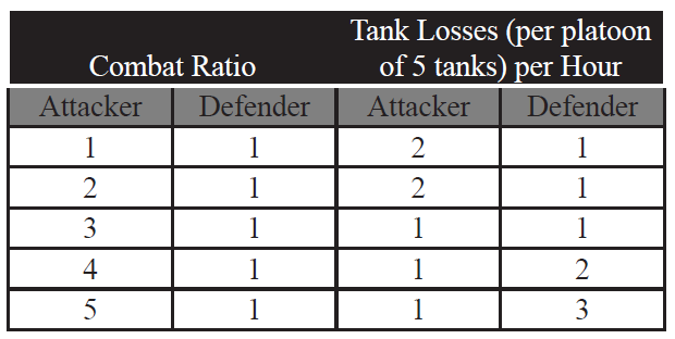
Finally, there is a version of the rule that dates from the 1967 Maneuver Control manual that only applies to armor that shows:
As the RAND construct also applies to equipment losses, then this formulation is directly comparable to the RAND construct.
Therefore, we have three basic versions of the 3-to-1 rule as it applies to casualties and/or equipment losses. First, there is a rule that states that there is an even fractional loss ratio at 3-to-1 (the RAND version), Second, there is a rule that states that at 3-to-1, the attacker will suffer one-third the losses of the defender. And third, there is a rule that states that at 3-to-1, the attacker and defender will suffer the same losses as the defender. Furthermore, these examples are highly contradictory, with either the attacker suffering three times the losses of the defender, the attacker suffering the same losses as the defender, or the attacker suffering 1/3 the losses of the defender.
Therefore, what we will examine here is the relationship between force ratios and exchange ratios. In this case, we will first look at The Dupuy Institute’s Battles Database (BaDB), which covers 243 battles from 1600 to 1900. We will chart on the y-axis the force ratio as measured by a count of the number of people on each side of the forces deployed for battle. The force ratio is the number of attackers divided by the number of defenders. On the x-axis is the exchange ratio, which is a measured by a count of the number of people on each side who were killed, wounded, missing or captured during that battle. It does not include disease and non-battle injuries. Again, it is calculated by dividing the total attacker casualties by the total defender casualties. The results are provided below:
As can be seen, there are a few extreme outliers among these 243 data points. The most extreme, the Battle of Tippennuir (l Sep 1644), in which an English Royalist force under Montrose routed an attack by Scottish Covenanter militia, causing about 3,000 casualties to the Scots in exchange for a single (allegedly self-inflicted) casualty to the Royalists, was removed from the chart. This 3,000-to-1 loss ratio was deemed too great an outlier to be of value in the analysis.
As it is, the vast majority of cases are clumped down into the corner of the graph with only a few scattered data points outside of that clumping. If one did try to establish some form of curvilinear relationship, one would end up drawing a hyperbola. It is worthwhile to look inside that clump of data to see what it shows. Therefore, we will look at the graph truncated so as to show only force ratios at or below 20-to-1 and exchange rations at or below 20-to-1.
Again, the data remains clustered in one corner with the outlying data points again pointing to a hyperbola as the only real fitting curvilinear relationship. Let’s look at little deeper into the data by truncating the data on 6-to-1 for both force ratios and exchange ratios. As can be seen, if the RAND version of the 3-to-1 rule is correct, then the data should show at 3-to-1 force ratio a 3-to-1 casualty exchange ratio. There is only one data point that comes close to this out of the 243 points we examined.
If the FM 105-5 version of the rule as it applies to armor is correct, then the data should show that at 3-to-1 force ratio there is a 1-to-1 casualty exchange ratio, at a 4-to-1 force ratio a 1-to-2 casualty exchange ratio, and at a 5-to-1 force ratio a 1-to-3 casualty exchange ratio. Of course, there is no armor in these pre-WW I engagements, but again no such exchange pattern does appear.
If the 1958 version of the FM 105-5 rule as it applies to casualties is correct, then the data should show that at a 3-to-1 force ratio there is 0.33-to-1 casualty exchange ratio, at a 4-to-1 force ratio a .25-to-1 casualty exchange ratio, and at a 5-to-1 force ratio a 0.20-to-5 casualty exchange ratio. As can be seen, there is not much indication of this pattern, or for that matter any of the three patterns.
Still, such a construct may not be relevant to data before 1900. For example, Lanchester claimed in 1914 in Chapter V, “The Principal of Concentration,” of his book Aircraft in Warfare, that there is greater advantage to be gained in modern warfare from concentration of fire.[3] Therefore, we will tap our more modern Division-Level Engagement Database (DLEDB) of 675 engagements, of which 628 have force ratios and exchange ratios calculated for them. These 628 cases are then placed on a scattergram to see if we can detect any similar patterns.
Even though this data covers from 1904 to 1991, with the vast majority of the data coming from engagements after 1940, one again sees the same pattern as with the data from 1600-1900. If there is a curvilinear relationship, it is again a hyperbola. As before, it is useful to look into the mass of data clustered into the corner by truncating the force and exchange ratios at 20-to-1. This produces the following:
Again, one sees the data clustered in the corner, with any curvilinear relationship again being a hyperbola. A look at the data further truncated to a 10-to-1 force or exchange ratio does not yield anything more revealing.
And, if this data is truncated to show only 5-to-1 force ratio and exchange ratios, one again sees:
Again, this data appears to be mostly just noise, with no clear patterns here that support any of the three constructs. In the case of the RAND version of the 3-to-1 rule, there is again only one data point (out of 628) that is anywhere close to the crossover point (even fractional exchange rate) that RAND postulates. In fact, it almost looks like the data conspires to make sure it leaves a noticeable “hole” at that point. The other postulated versions of the 3-to-1 rules are also given no support in these charts.
While we can attempt to torture the data to find a better fit, or can try to argue that the patterns are obscured by various factors that have not been considered, we do not believe that such a clear pattern and relationship exists. More advanced mathematical methods may show such a pattern, but to date such attempts have not ferreted out these alleged patterns. For example, we refer the reader to Janice Fain’s article on Lanchester equations, The Dupuy Institute’s Capture Rate Study, Phase I & II, or any number of other studies that have looked at Lanchester.[4]
The fundamental problem is that there does not appear to be a direct cause and effect between force ratios and exchange ratios. It appears to be an indirect relationship in the sense that force ratios are one of several independent variables that determine the outcome of an engagement, and the nature of that outcome helps determines the casualties. As such, there is a more complex set of interrelationships that have not yet been fully explored in any study that we know of, although it is briefly addressed in our Capture Rate Study, Phase I & II.
[3] F. W. Lanchester, Aircraft in Warfare: The Dawn of the Fourth Arm (Lanchester Press Incorporated, Sunnyvale, Calif., 1995), 46-60. One notes that Lanchester provided no data to support these claims, but relied upon an intellectual argument based upon a gross misunderstanding of ancient warfare.
Thanks to a comment made on one of our posts, I recently became aware of a 17 page discussion thread on combat results tables (CRT) that is worth reading. It is here:
By default, much of their discussion of data centers around analysis based upon Trevor Dupuy’s writing, the CBD90 database, the Ardennes Campaign Simulation Data Base (ACSDB), the Kursk Data Base (KDB) and my book War by Numbers. I was not aware of this discussion until yesterday even though the thread was started in 2015 and continues to this year (War by Numbers was published in 2017 so does not appear until the end of page 5 of the thread).
The CBD90 was developed from a Dupuy research effort in the 1980s eventually codified as the Land Warfare Data Base (LWDB). Dupuy’s research was programmed with errors by the government to create the CBD90. A lot of the analysis in my book was based upon a greatly expanded and corrected version of the LWDB. I was the program manager for both the ACSDB and the KDB, and of course, the updated versions of our DuWar suite of combat databases.
There are about a hundred comments I could make to this thread, some in agreement and some in disagreement, but then I would not get my next book finished, so I will refrain. This does not stop me from posting a link:
[This post was originally published on 13 December 2017]
And then…..we discovered the existence of a significant missing study that we wanted to see.
Around 2000, the Center for Army Analysis (CAA) contracted The Dupuy Institute to conduct an analysis of how to represent urban warfare in combat models. This was the first work we had ever done on urban warfare, so…….we first started our literature search. While there was a lot of impressionistic stuff gathered from reading about Stalingrad and watching field exercises, there was little hard data or analysis. Simply no one had ever done any analysis of the nature of urban warfare.
But, on the board of directors of The Dupuy Institute was a grand old gentleman called John Kettelle. He had previously been the president of Ketron, an operations research company that he had founded. Kettelle had been around the business for a while, having been an office mate of Kimball, of Morse and Kimbell fame (the people who wrote the original U.S. Operations Research “textbook” in 1951: Methods of Operations Research). He is here: https://www.adventfuneral.com/services/john-dunster-kettelle-jr.htm?wpmp_switcher=mobile
John had mentioned several times a massive study on urban warfare that he had done for the U.S. Army in the 1970s. He had mentioned details of it, including that it was worked on by his staff over the course of several years, consisted of several volumes, looked into operations in Stalingrad, was pretty extensive and exhaustive, and had a civil disturbance component to it that he claimed was there at the request of the Nixon White House. John Kettelle sold off his company Ketron in the 1990s and was now semi-retired.
So, I asked John Kettelle where his study was. He said he did not know. He called over to the surviving elements of Ketron and they did not have a copy. Apparently significant parts of the study were classified. In our review of the urban warfare literature around 2000 we found no mention of the study or indications that anyone had seen or drawn any references from it.
This was probably the first extensive study ever done on urban warfare. It employed at least a half-dozen people for multiple years. Clearly the U.S. Army spent several million of our hard earned tax dollars on it…..yet is was not being used and could not be found. It was not listed in DTIC, NTIS, on the web, nor was it in Ketron’s files, and John Kettelle did not have a copy of it. It was lost !!!
So, we proceeded with our urban warfare studies independent of past research and ended up doing three reports on the subject. Theses studies are discussed in two chapters of my book War by Numbers.
As the Ketron urban warfare study was classified, there were probably copies of it in classified U.S. Army command files in the 1970s. If these files have been properly retired then these classified files may exist in the archives. At some point, they may be declassified. At some point the study may be re-discovered. But……the U.S. Army after spending millions for this study, preceded to obtain no benefit from the study in the late 1990s, when a lot of people re-opened the issue of urban warfare. This would have certainly been a useful study, especially as much of what the Army, RAND and others were discussing at the time was not based upon hard data and was often dead wrong.
This may be a case of the U.S. Army having to re-invent the wheel because it has not done a good job of protecting and disseminating its studies and analysis. This seems to particularly be a problem with studies that were done by contractors that have gone out of business. Keep in mind, we were doing our urban warfare work for the Centerfor Army Analysis. As a minimum, they should have had a copy of it.
More on the QJM/TNDM Italian Battles by Richard C. Anderson, Jr.
In regard to Niklas Zetterling’s article and Christopher Lawrence’s response (Newsletter Volume 1, Number 6) [and Christopher Lawrence’s 2018 addendum] I would like to add a few observations of my own. Recently I have had occasion to revisit the Allied and German records for Italy in general and for the Battle of Salerno in particular. What I found is relevant in both an analytical and an historical sense.
The Salerno Order of Battle
The first and most evident observation that I was able to make of the Allied and German Order of Battle for the Salerno engagements was that it was incorrect. The following observations all relate to the table found on page 25 of Volume 1, Number 6.
The divisional totals are misleading. The U.S. had one infantry division (the 36th) and two-thirds of a second (the 45th, minus the 180th RCT [Regimental Combat Team] and one battalion of the 157th Infantry) available during the major stages of the battle (9-15 September 1943). The 82nd Airborne Division was represented solely by elements of two parachute infantry regiments that were dropped as emergency reinforcements on 13-14 September. The British 7th Armored Division did not begin to arrive until 15-16 September and was not fully closed in the beachhead until 18-19 September.
The German situation was more complicated. Only a single panzer division, the 16th, under the command of the LXXVI Panzer Corps was present on 9 September. On 10 September elements of the Hermann Goring Parachute Panzer Division, with elements of the 15th Panzergrenadier Division under tactical command, began arriving from the vicinity of Naples. Major elements of the Herman Goring Division (with its subordinated elements of the 15th Panzergrenadier Division) were in place and had relieved elements of the 16th Panzer Division opposing the British beaches by 11 September. At the same time the 29th Panzergrenandier Division began arriving from Calabria and took up positions opposite the U.S. 36th Divisions in and south of Altavilla, again relieving elements of the 16th Panzer Division. By 11-12 September the German forces in the northern sector of the beachhead were under the command of the XIV Panzer Corps (Herman Goring Division (-), elements of the 15th Panzergrenadier Division and elements of the 3rd Panzergrenadier Division), while the LXXVI Panzer Corps commanded the 16th Panzer Division, 29th Panzergrenadier Division, and elements of the 26th Panzer Division. Unfortunately for the Germans the 16th Panzer Division’s zone was split by the boundary between the XIV and LXXVI Corps, both of whom appear to have had operational control over different elements of the division. Needless to say, the German command and control problems in this action were tremendous.[1]
The artillery totals given in the table are almost inexplicable. The numbers of SP [self-propelled] 75mm howitzers is a bit fuzzy, inasmuch as this was a non-standardized weapon on a half-track chassis. It was allocated to the infantry regimental cannon company (6 tubes) and was also issued to tank and tank destroyer battalions as a stopgap until purpose-designed systems could be brought into production. The 105mm SP was also present on a half-track chassis in the regimental cannon company (2 tubes) and on a full-track chassis in the armored field artillery battalion (18 tubes). The towed 105mm artillery was present in the five field artillery battalions present of the 36th and 45th divisions and in a single non-divisional battalion assigned to the VI Corps. The 155mm howitzers were only present in the two divisional field artillery battalions, the general support artillery assigned to the VI Corps, the 36th Field Artillery Regiment, did not arrive until 16 September. No 155mm gun battalions landed in Italy until October 1943. The U.S. artillery figures should approximately be as follows:
75mm Howitzer (SP)
2 per infantry battalion
28
6 per tank battalion
12
Total
40
105mm Howitzer (SP)
2 per infantry regiment
10
1 armored FA battalion[2]
18
5 divisional FA battalions
60
1 non-divisional FA battalion
12
Total
100
155mm Howitzer
2 divisional FA battalions
24
3″ Tank Destroyer
3 battalions
108
Thus, the U.S. artillery strength is approximately 272 versus 525 as given in the chart.
The British artillery figures are also suspect. Each of the British divisions present, the 46th and 56th, had three regiments (battalions in U.S. parlance) of 25-pounder gun-howitzers for a total of 72 per division. There is no evidence of the presence of the British 3-inch howitzer, except possibly on a tank chassis in the support tank role attached to the tank troop headquarters of the armor regiment (battalion) attached to the X Corps (possibly 8 tubes). The X Corps had a single medium regiment (battalion) attached with either 4.5 inch guns or 5.5 inch gun-howitzers or a mixture of the two (16 tubes). The British did not have any 7.2 inch howitzers or 155mm guns at Salerno. I do not know where the figure for British 75mm howitzers is from, although it is possible that some may have been present with the corps armored car regiment.
Thus the British artillery strength is approximately 168 versus 321 as given in the chart.
The German artillery types are highly suspect. As Niklas Zetterling deduced, there was no German corps or army artillery present at Salemo. Neither the XIV or LXXVI Corps had Heeres (army) artillery attached. The two battalions of the 7lst Nebelwerfer regiment and one battery of 170mm guns (previously attached to the 15th Panzergrenadier Division) were all out of action, refurbishing and replenishing equipment in the vicinity of Naples. However, U.S. intelligence sources located 42 Italian coastal gun positions, including three 149mm (not 132mm) railway guns defending the beaches. These positions were taken over by German personnel on the night before the invasion. That they fired at all in the circumstances is a comment on the professionalism of the German Army. The remaining German artillery available was with the divisional elements that arrived to defend against the invasion forces. The following artillery strengths are known for the German forces at Salerno:
501st Army Flak Battalion (probably 20mm and 37mm AA only)
I/49th Flak Battalion (probably 8 88mm AA guns)
Thus, German artillery strength is about 342 tubes versus 394 as given in the chart.[3]
Armor strengths are equally suspect for both the Allied and German forces. It should be noted however, that the original QJM database considered wheeled armored cars to be the equivalent of a light tank.
Only two U.S. armor battalions were assigned to the initial invasion force, with a total of 108 medium and 34 light tanks. The British X Corps had a single armor regiment (battalion) assigned with approximately 67 medium and 10 light tanks. Thus, the Allies had some 175 medium tanks versus 488 as given in the chart and 44 light tanks versus 236 (including an unknown number of armored cars) as given in the chart.
German armor strength was as follows (operational/in repair as of the date given):
16th Panzer Division (8 September):
7/0 Panzer III flamethrower tanks
12/0 Panzer IV short
86/6 Panzer IV long
37/3 assault guns
29th Panzergrenadier Division (1 September):
32/5 assault guns
17/4 SP antitank
3/0 Panzer III
26th Panzer Division (5 September):
11/? assault guns
10/? Panzer III
Herman Goering Parachute Panzer Division (7 September):
5/? Panzer IV short
11/? Panzer IV long
5/? Panzer III long
1/? Panzer III 75mm
21/? assault guns
3/? SP antitank
15th Panzergrenadier Division (8 September):
6/? Panzer IV long
18/? assault guns
Total 285/18 medium tanks, SP anti-tank, and assault guns. This number actually agrees very well with the 290 medium tanks given in the chart. I have not looked closely at the number of German armored cars but suspect that it is fairly close to that given in the charts.
In general it appears that the original QJM Database got the numbers of major items of equipment right for the Germans, even if it flubbed on the details. On the other hand, the numbers and details are highly suspect for the Allied major items of equipment. Just as a first order “guestimate” I would say that this probably reduces the German CEV to some extent; however, missing from the formula is the Allied naval gunfire support which, although negligible in impact in the initial stages of the battle, had a strong influence on the later stages of the battle.
Hopefully, with a little more research and time, we will be able to go back and revalidate these engagements. In the meantime I hope that this has clarified some of the questions raised about the Italian QJM Database.
NOTES
[1] Exacerbating the German command and control problems was the fact that the Tenth Army, which was in overall command of the XIV Panzer Corps and LXXVI Panzer Corps, had only been in existence for about six weeks. The army’s signal regiment was only partly organized and its quartermaster services were almost nonexistent.
[2] Arrived 13 September, 1 battery in action 13-15 September.
[3] However, the number given for the 29th Panzergrenadier Division appears to be suspiciously high and is not well defined. Hopefully further research may clarify the status of this division.
Shawn likes to post up on the blog old articles from The International TNDM Newsletter. The previous blog post was one such article I wrote in 1997 (he posted it under my name…although he put together the post). This is the first time I have read it since say….1997. A few comments:
In fact, we did go back in systematically review and correct all the Italian engagements. This was primarily done by Richard Anderson from German records and UK records. All the UK engagements were revised as were many of the other Italian Campaign records. In fact, we ended up revising at least half of the WWII engagements in the Land Warfare Data Base (LWDB).
We did greatly expand our collection of data, to over 1,200 engagements, including 752 in a division-level engagement database. Basically we doubled the size of the database (and placed it in Access).
Using this more powerful data collection, I then re-shot the analysis of combat effectiveness. I did not use any modeling structure, but simply just used basic statistics. This effort again showed a performance difference in combat in Italy between the Germans, the Americans and the British. This is discussed in War by Numbers, pages 19-31.
We did actually re-validate the TNDM. The results of this validation are published in War by Numbers, pages 299-324. They were separately validated at corps-level (WWII), division-level (WWII) and at Battalion-level (WWI, WWII and post-WWII).
War by Numbers also includes a detailed discussion of differences in casualty reporting between nations (pages 202-205) and between services (pages 193-202).
We have never done an analysis of the value of terrain using our larger more robust databases, although this is on my short-list of things to do. This is expected to be part of War by Numbers II, if I get around to writing it.
We have done no significant re-design of the TNDM.
Anyhow, that is some of what we have been doing in the intervening 20 years since I wrote that article.
Response to Niklas Zetterling’s Article by Christopher A. Lawrence
Mr. Zetterling is currently a professor at the Swedish War College and previously worked at the Swedish National Defense Research Establishment. As I have been having an ongoing dialogue with Prof. Zetterling on the Battle of Kursk, I have had the opportunity to witness his approach to researching historical data and the depth of research. I would recommend that all of our readers take a look at his recent article in the Journal of Slavic Military Studies entitled “Loss Rates on the Eastern Front during World War II.” Mr. Zetterling does his German research directly from the Captured German Military Records by purchasing the rolls of microfilm from the US National Archives. He is using the same German data sources that we are. Let me attempt to address his comments section by section:
The Database on Italy 1943-44:
Unfortunately, the Italian combat data was one of the early HERO research projects, with the results first published in 1971. I do not know who worked on it nor the specifics of how it was done. There are references to the Captured German Records, but significantly, they only reference division files for these battles. While I have not had the time to review Prof. Zetterling‘s review of the original research. I do know that some of our researchers have complained about parts of the Italian data. From what I’ve seen, it looks like the original HERO researchers didn’t look into the Corps and Army files, and assumed what the attached Corps artillery strengths were. Sloppy research is embarrassing, although it does occur, especially when working under severe financial constraints (for example, our Battalion-level Operations Database). If the research is sloppy or hurried, or done from secondary sources, then hopefully the errors are random, and will effectively counterbalance each other, and not change the results of the analysis. If the errors are all in one direction, then this will produce a biased result.
I have no basis to believe that Prof. Zetterling’s criticism is wrong, and do have many reasons to believe that it is correct. Until l can take the time to go through the Corps and Army files, I intend to operate under the assumption that Prof. Zetterling’s corrections are good. At some point I will need to go back through the Italian Campaign data and correct it and update the Land Warfare Database. I did compare Prof. Zetterling‘s list of battles with what was declared to be the forces involved in the battle (according to the Combat Data Subscription Service) and they show the following attached artillery:
It is clear that the battles were based on the assumption that here was Corps-level German artillery. A strength comparison between the two sides is displayed in the chart on the next page.
The Result Formula:
CEV is calculated from three factors. Therefore a consistent 20% error in casualties will result in something less than a 20% error in CEV. The mission effectiveness factor is indeed very “fuzzy,” and these is simply no systematic method or guidance in its application. Sometimes, it is not based upon the assigned mission of the unit, but its perceived mission based upon the analyst’s interpretation. But, while l have the same problems with the mission accomplishment scores as Mr. Zetterling, I do not have a good replacement. Considering the nature of warfare, I would hate to create CEVs without it. Of course, Trevor Dupuy was experimenting with creating CEVs just from casualty effectiveness, and by averaging his two CEV scores (CEVt and CEVI) he heavily weighted the CEV calculation for the TNDM towards measuring primarily casualty effectiveness (see the article in issue 5 of the Newsletter, “Numerical Adjustment of CEV Results: Averages and Means“). At this point, I would like to produce a new, single formula for CEV to replace the current two and its averaging methodology. I am open to suggestions for this.
Supply Situation:
The different ammunition usage rate of the German and US Armies is one of the reasons why adding a logistics module is high on my list of model corrections. This was discussed in Issue 2 of the Newsletter, “Developing a Logistics Model for the TNDM.” As Mr. Zetterling points out, “It is unlikely that an increase in artillery ammunition expenditure will result in a proportional increase in combat power. Rather it is more likely that there is some kind of diminished return with increased expenditure.” This parallels what l expressed in point 12 of that article: “It is suspected that this increase [in OLIs] will not be linear.”
The CEV does include “logistics.” So in effect, if one had a good logistics module, the difference in logistics would be accounted for, and the Germans (after logistics is taken into account) may indeed have a higher CEV.
General Problems with Non-Divisional Units Tooth-to-Tail Ratio
Point taken. The engagements used to test the TNDM have been gathered over a period of over 25 years, by different researchers and controlled by different management. What is counted when and where does change from one group of engagements to the next. While l do think this has not had a significant result on the model outcomes, it is “sloppy” and needs to be addressed.
The Effects of Defensive Posture
This is a very good point. If the budget was available, my first step in “redesigning” the TNDM would be to try to measure the effects of terrain on combat through the use of a large LWDB-type database and regression analysis. I have always felt that with enough engagements, one could produce reliable values for these figures based upon something other than judgement. Prof. Zetterling’s proposed methodology is also a good approach, easier to do, and more likely to get a conclusive result. I intend to add this to my list of model improvements.
Conclusions
There is one other problem with the Italian data that Prof. Zetterling did not address. This was that the Germans and the Allies had different reporting systems for casualties. Quite simply, the Germans did not report as casualties those people who were lightly wounded and treated and returned to duty from the divisional aid station. The United States and England did. This shows up when one compares the wounded to killed ratios of the various armies, with the Germans usually having in the range of 3 to 4 wounded for every one killed, while the allies tend to have 4 to 5 wounded for every one killed. Basically, when comparing the two reports, the Germans “undercount” their casualties by around 17 to 20%. Therefore, one probably needs to use a multiplier of 20 to 25% to match the two casualty systems. This was not taken into account in any the work HERO did.
Because Trevor Dupuy used three factors for measuring his CEV, this error certainly resulted in a slightly higher CEV for the Germans than should have been the case, but not a 20% increase. As Prof. Zetterling points out, the correction of the count of artillery pieces should result in a higher CEV than Col. Dupuy calculated. Finally, if Col. Dupuy overrated the value of defensive terrain, then this may result in the German CEV being slightly lower.
As you may have noted in my list of improvements (Issue 2, “Planned Improvements to the TNDM”), I did list “revalidating” to the QJM Database. [NOTE: a summary of the QJM/TNDM validation efforts can be found here.] As part of that revalidation process, we would need to review the data used in the validation data base first, account for the casualty differences in the reporting systems, and determine if the model indeed overrates the effect of terrain on defense.
Perhaps one of the most debated results of the TNDM (and its predecessors) is the conclusion that the German ground forces on average enjoyed a measurable qualitative superiority over its US and British opponents. This was largely the result of calculations on situations in Italy in 1943-44, even though further engagements have been added since the results were first presented. The calculated German superiority over the Red Army, despite the much smaller number of engagements, has not aroused as much opposition. Similarly, the calculated Israeli effectiveness superiority over its enemies seems to have surprised few.
However, there are objections to the calculations on the engagements in Italy 1943. These concern primarily the database, but there are also some questions to be raised against the way some of the calculations have been made, which may possibly have consequences for the TNDM.
Here it is suggested that the German CEV [combat effectiveness value] superiority was higher than originally calculated. There are a number of flaws in the original calculations, each of which will be discussed separately below. With the exception of one issue, all of them, if corrected, tend to give a higher German CEV.
The Database on Italy 1943-44
According to the database the German divisions had considerable fire support from GHQ artillery units. This is the only possible conclusion from the fact that several pieces of the types 15cm gun, 17cm gun, 21cm gun, and 15cm and 21cm Nebelwerfer are included in the data for individual engagements. These types of guns were almost exclusively confined to GHQ units. An example from the database are the three engagements Port of Salerno, Amphitheater, and Sele-Calore Corridor. These take place simultaneously (9-11 September 1943) with the German 16th Pz Div on the Axis side in all of them (no other division is included in the battles). Judging from the manpower figures, it seems to have been assumed that the division participated with one quarter of its strength in each of the two former battles and half its strength in the latter. According to the database, the number of guns were:
15cm gun
28
17cm gun
12
21cm gun
12
15cm NbW
27
21cm NbW
21
This would indicate that the 16th Pz Div was supported by the equivalent of more than five non-divisional artillery battalions. For the German army this is a suspiciously high number, usually there were rather something like one GHQ artillery battalion for each division, or even less. Research in the German Military Archives confirmed that the number of GHQ artillery units was far less than indicated in the HERO database. Among the useful documents found were a map showing the dispositions of 10th Army artillery units. This showed clearly that there was only one non-divisional artillery unit south of Rome at the time of the Salerno landings, the III/71 Nebelwerfer Battalion. Also the 557th Artillery Battalion (17cm gun) was present, it was included in the artillery regiment (33rd Artillery Regiment) of 15th Panzergrenadier Division during the second half of 1943. Thus the number of German artillery pieces in these engagements is exaggerated to an extent that cannot be considered insignificant. Since OLI values for artillery usually constitute a significant share of the total OLI of a force in the TNDM, errors in artillery strength cannot be dismissed easily.
While the example above is but one, further archival research has shown that the same kind of error occurs in all the engagements in September and October 1943. It has not been possible to check the engagements later during 1943, but a pattern can be recognized. The ratio between the numbers of various types of GHQ artillery pieces does not change much from battle to battle. It seems that when the database was developed, the researchers worked with the assumption that the German corps and army organizations had organic artillery, and this assumption may have been used as a “rule of thumb.” This is wrong, however; only artillery staffs, command and control units were included in the corps and army organizations, not firing units. Consequently we have a systematic error, which cannot be corrected without changing the contents of the database. It is worth emphasizing that we are discussing an exaggeration of German artillery strength of about 100%, which certainly is significant. Comparing the available archival records with the database also reveals errors in numbers of tanks and antitank guns, but these are much smaller than the errors in artillery strength. Again these errors do always inflate the German strength in those engagements l have been able to check against archival records. These errors tend to inflate German numerical strength, which of course affects CEV calculations. But there are further objections to the CEV calculations.
The Result Formula
The “result formula” weighs together three factors: casualties inflicted, distance advanced, and mission accomplishment. It seems that the first two do not raise many objections, even though the relative weight of them may always be subject to argumentation.
The third factor, mission accomplishment, is more dubious however. At first glance it may seem to be natural to include such a factor. Alter all, a combat unit is supposed to accomplish the missions given to it. However, whether a unit accomplishes its mission or not depends both on its own qualities as well as the realism of the mission assigned. Thus the mission accomplishment factor may reflect the qualities of the combat unit as well as the higher HQs and the general strategic situation. As an example, the Rapido crossing by the U.S. 36th Infantry Division can serve. The division did not accomplish its mission, but whether the mission was realistic, given the circumstances, is dubious. Similarly many German units did probably, in many situations, receive unrealistic missions, particularly during the last two years of the war (when most of the engagements in the database were fought). A more extreme example of situations in which unrealistic missions were given is the battle in Belorussia, June-July 1944, where German units were regularly given impossible missions. Possibly it is a general trend that the side which is fighting at a strategic disadvantage is more prone to give its combat units unrealistic missions.
On the other hand it is quite clear that the mission assigned may well affect both the casualty rates and advance rates. If, for example, the defender has a withdrawal mission, advance may become higher than if the mission was to defend resolutely. This must however not necessarily be handled by including a missions factor in a result formula.
I have made some tentative runs with the TNDM, testing with various CEV values to see which value produced an outcome in terms of casualties and ground gained as near as possible to the historical result. The results of these runs are very preliminary, but the tendency is that higher German CEVs produce more historical outcomes, particularly concerning combat.
Supply Situation
According to scattered information available in published literature, the U.S. artillery fired more shells per day per gun than did German artillery. In Normandy, US 155mm M1 howitzers fired 28.4 rounds per day during July, while August showed slightly lower consumption, 18 rounds per day. For the 105mm M2 howitzer the corresponding figures were 40.8 and 27.4. This can be compared to a German OKH study which, based on the experiences in Russia 1941-43, suggested that consumption of 105mm howitzer ammunition was about 13-22 rounds per gun per day, depending on the strength of the opposition encountered. For the 150mm howitzer the figures were 12-15.
While these figures should not be taken too seriously, as they are not from primary sources and they do also reflect the conditions in different theaters, they do at least indicate that it cannot be taken for granted that ammunition expenditure is proportional to the number of gun barrels. In fact there also exist further indications that Allied ammunition expenditure was greater than the German. Several German reports from Normandy indicate that they were astonished by the Allied ammunition expenditure.
It is unlikely that an increase in artillery ammunition expenditure will result in a proportional increase combat power. Rather it is more likely that there is some kind of diminished return with increased expenditure.
General Problems with Non-Divisional Units
A division usually (but not necessarily) includes various support services, such as maintenance, supply, and medical services. Non-divisional combat units have to a greater extent to rely on corps and army for such support. This makes it complicated to include such units, since when entering, for example, the manpower strength and truck strength in the TNDM, it is difficult to assess their contribution to the overall numbers.
Furthermore, the amount of such forces is not equal on the German and Allied sides. In general the Allied divisional slice was far greater than the German. In Normandy the US forces on 25 July 1944 had 812,000 men on the Continent, while the number of divisions was 18 (including the 5th Armored, which was in the process of landing on the 25th). This gives a divisional slice of 45,000 men. By comparison the German 7th Army mustered 16 divisions and 231,000 men on 1 June 1944, giving a slice of 14,437 men per division. The main explanation for the difference is the non-divisional combat units and the logistical organization to support them. In general, non-divisional combat units are composed of powerful, but supply-consuming, types like armor, artillery, antitank and antiaircraft. Thus their contribution to combat power and strain on the logistical apparatus is considerable. However I do not believe that the supporting units’ manpower and vehicles have been included in TNDM calculations.
There are however further problems with non-divisional units. While the whereabouts of tank and tank destroyer units can usually be established with sufficient certainty, artillery can be much harder to pin down to a specific division engagement. This is of course a greater problem when the geographical extent of a battle is small.
Tooth-to-Tail Ratio
Above was discussed the lack of support units in non-divisional combat units. One effect of this is to create a force with more OLI per man. This is the result of the unit‘s “tail” belonging to some other part of the military organization.
In the TNDM there is a mobility formula, which tends to favor units with many weapons and vehicles compared to the number of men. This became apparent when I was performing a great number of TNDM runs on engagements between Swedish brigades and Soviet regiments. The Soviet regiments usually contained rather few men, but still had many AFVs, artillery tubes, AT weapons, etc. The Mobility Formula in TNDM favors such units. However, I do not think this reflects any phenomenon in the real world. The Soviet penchant for lean combat units, with supply, maintenance, and other services provided by higher echelons, is not a more effective solution in general, but perhaps better suited to the particular constraints they were experiencing when forming units, training men, etc. In effect these services were existing in the Soviet army too, but formally not with the combat units.
This problem is to some extent reminiscent to how density is calculated (a problem discussed by Chris Lawrence in a recent issue of the Newsletter). It is comparatively easy to define the frontal limit of the deployment area of force, and it is relatively easy to define the lateral limits too. It is, however, much more difficult to say where the rear limit of a force is located.
When entering forces in the TNDM a rear limit is, perhaps unintentionally, drawn. But if the combat unit includes support units, the rear limit is pushed farther back compared to a force whose combat units are well separated from support units.
To what extent this affects the CEV calculations is unclear. Using the original database values, the German forces are perhaps given too high combat strength when the great number of GHQ artillery units is included. On the other hand, if the GHQ artillery units are not included, the opposite may be true.
The Effects of Defensive Posture
The posture factors are difficult to analyze, since they alone do not portray the advantages of defensive position. Such effects are also included in terrain factors.
It seems that the numerical values for these factors were assigned on the basis of professional judgement. However, when the QJM was developed, it seems that the developers did not assume the German CEV superiority. Rather, the German CEV superiority seems to have been discovered later. It is possible that the professional judgement was about as wrong on the issue of posture effects as they were on CEV. Since the British and American forces were predominantly on the offensive, while the Germans mainly defended themselves, a German CEV superiority may, at least partly, be hidden in two high effects for defensive posture.
When using corrected input data on the 20 situations in Italy September-October 1943, there is a tendency that the German CEV is higher when they attack. Such a tendency is also discernible in the engagements presented in Hitler’s Last Gamble. Appendix H, even though the number of engagements in the latter case is very small.
As it stands now this is not really more than a hypothesis, since it will take an analysis of a greater number of engagements to confirm it. However, if such an analysis is done, it must be done using several sets of data. German and Allied attacks must be analyzed separately, and preferably the data would be separated further into sets for each relevant terrain type. Since the effects of the defensive posture are intertwined with terrain factors, it is very much possible that the factors may be correct for certain terrain types, while they are wrong for others. It may also be that the factors can be different for various opponents (due to differences in training, doctrine, etc.). It is also possible that the factors are different if the forces are predominantly composed of armor units or mainly of infantry.
One further problem with the effects of defensive position is that it is probably strongly affected by the density of forces. It is likely that the main effect of the density of forces is the inability to use effectively all the forces involved. Thus it may be that this factor will not influence the outcome except when the density is comparatively high. However, what can be regarded as “high” is probably much dependent on terrain, road net quality, and the cross-country mobility of the forces.
Conclusions
While the TNDM has been criticized here, it is also fitting to praise the model. The very fact that it can be criticized in this way is a testimony to its openness. In a sense a model is also a theory, and to use Popperian terminology, the TNDM is also very testable.
It should also be emphasized that the greatest errors are probably those in the database. As previously stated, I can only conclude safely that the data on the engagements in Italy in 1943 are wrong; later engagements have not yet been checked against archival documents. Overall the errors do not represent a dramatic change in the CEV values. Rather, the Germans seem to have (in Italy 1943) a superiority on the order of 1.4-1.5, compared to an original figure of 1.2-1.3.
During September and October 1943, almost all the German divisions in southern Italy were mechanized or parachute divisions. This may have contributed to a higher German CEV. Thus it is not certain that the conclusions arrived at here are valid for German forces in general, even though this factor should not be exaggerated, since many of the German divisions in Italy were either newly raised (e.g., 26th Panzer Division) or rebuilt after the Stalingrad disaster (16th Panzer Division plus 3rd and 29th Panzergrenadier Divisions) or the Tunisian debacle (15th Panzergrenadier Division).
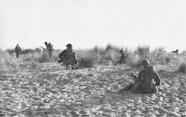
Jeffrey H Michaels, a Senior Lecturer in Defence Studies at the British the Joint Services Command and Staff College, has published a detailed look at how Hackett and several senior NATO and diplomatic colleagues constructed the scenario portrayed in the book. Scenario construction is an important aspect of institutional war gaming. A war game will only be as useful if the assumptions that underpin it are valid. As Michaels points out,
Regrettably, far too many scenarios and models, whether developed by military organizations, political scientists, or fiction writers, tend to focus their attention on the battlefield and the clash of armies, navies, air forces, and especially their weapons systems. By contrast, the broader context of the war – the reasons why hostilities erupted, the political and military objectives, the limits placed on military action, and so on – are given much less serious attention, often because they are viewed by the script-writers as a distraction from the main activity that occurs on the battlefield.
Modelers and war gamers always need to keep in mind the fundamental importance of context in designing their simulations.
It is quite easy to project how one weapon system might fare against another, but taken out of a broader strategic context, such a projection is practically meaningless (apart from its marketing value), or worse, misleading. In this sense, even if less entertaining or exciting, the degree of realism of the political aspects of the scenario, particularly policymakers’ rationality and cost-benefit calculus, and the key decisions that are taken about going to war, the objectives being sought, the limits placed on military action, and the willingness to incur the risks of escalation, should receive more critical attention than the purely battlefield dimensions of the future conflict.
These are crucially important points to consider when deciding how to asses the outcomes of hypothetical scenarios.
It is my understanding that he was the person who was responsible for making sure that DACM (Dupuy Air Combat Model) was funded by AFSC. He then retired from the Air Force in 1994. We completed the demonstration phase of the DACM and quite simply, there was no one left in the Air Force who was interested in funding it. So, work stopped. I never met General McInerney and was not involved in the marketing of the initial effort.
But, this is typical of the problems with doing business with the Pentagon, where an officer will take an interest in your work, generate funding for it, but by the time the first steps are completed, that officer has moved on to another assignment. This has happened to us with other projects. One of these efforts was a joint research project that was done by TDI and former Army surgeon on casualty rates. It was for J-4 of the Joint Staff. The project officer there was extremely interested and involved in the work, but then moved to another assignment. By the time we got original effort completed, the division was headed by an Air Force Colonel who appeared to be only interested in things that flew. Therefore, the project died (except that parts of it were used for Chapter 15: Casualties, pages 193-198, in War by Numbers).
Our experience in dealing with the U.S. defense establishment is that sometimes research efforts that takes longer than a few months will die……because the people interested in it have moved on. This sometimes leads to simple, short-term analysis and fewer properly funded long-term projects.
Consistent Scoring of Weapons and Aggregation of Forces: The Cornerstone of Dupuy’s Quantitative Analysis of Historical Land Battles by
James G. Taylor, PhD,
Dept. of Operations Research, Naval Postgraduate School
Introduction
Col. Trevor N. Dupuy was an American original, especially as regards the quantitative study of warfare. As with many prophets, he was not entirely appreciated in his own land, particularly its Military Operations Research (OR) community. However, after becoming rather familiar with the details of his mathematical modeling of ground combat based on historical data, I became aware of the basic scientific soundness of his approach. Unfortunately, his documentation of methodology was not always accepted by others, many of whom appeared to confuse lack of mathematical sophistication in his documentation with lack of scientific validity of his basic methodology.
The purpose of this brief paper is to review the salient points of Dupuy’s methodology from a system’s perspective, i.e., to view his methodology as a system, functioning as an organic whole to capture the essence of past combat experience (with an eye towards extrapolation into the future). The advantage of this perspective is that it immediately leads one to the conclusion that if one wants to use some functional relationship derived from Dupuy’s work, then one should use his methodologies for scoring weapons, aggregating forces, and adjusting for operational circumstances; since this consistency is the only guarantee of being able to reproduce historical results and to project them into the future.
Implications (of this system’s perspective on Dupuy’s work) for current DOD models will be discussed. In particular, the Military OR community has developed quantitative methods for imputing values to weapon systems based on their attrition capability against opposing forces and force interactions.[1] One such approach is the so-called antipotential-potential method[2] used in TACWAR[3] to score weapons. However, one should not expect such scores to provide valid casualty estimates when combined with historically derived functional relationships such as the so-called ATLAS casualty-rate curves[4] used in TACWAR, because a different “yard-stick” (i.e. measuring system for estimating the relative combat potential of opposing forces) was used to develop such a curve.
Overview of Dupuy’s Approach
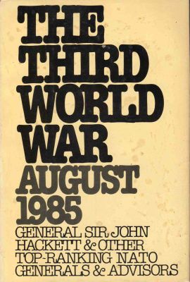
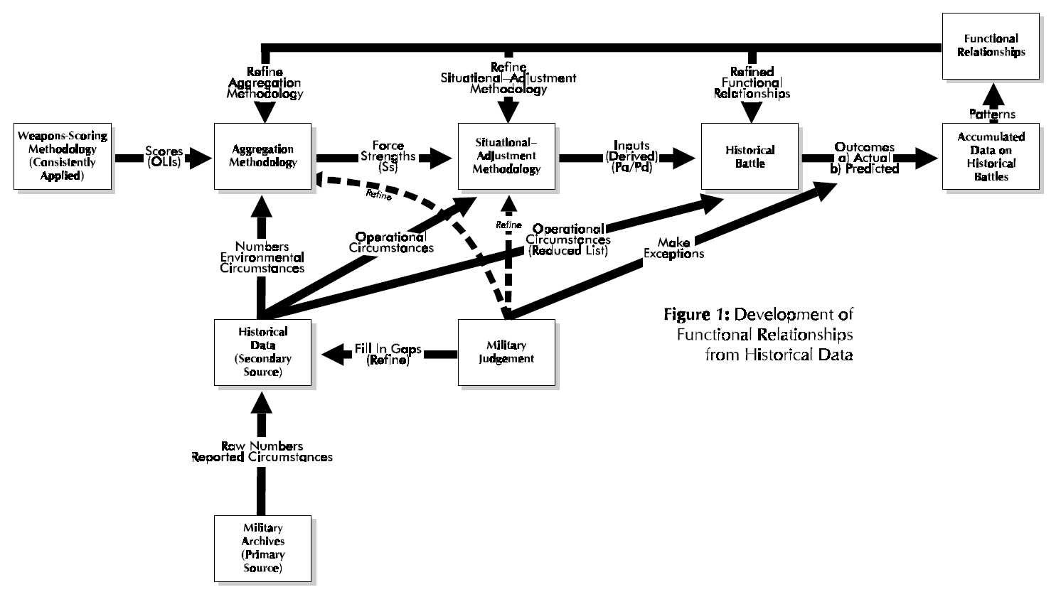
This section briefly outlines the salient features of Dupuy’s approach to the quantitative analysis and modeling of ground combat as embodied in his Tactical Numerical Deterministic Model (TNDM) and its predecessor the Quantified Judgment Model (QJM). The interested reader can find details in Dupuy [1979] (see also Dupuy [1985][5], [1987], [1990]). Here we will view Dupuy’s methodology from a system approach, which seeks to discern its various components and their interactions and to view these components as an organic whole. Essentially Dupuy’s approach involves the development of functional relationships from historical combat data (see Fig. 1) and then using these functional relationships to model future combat (see Fig, 2).
At the heart of Dupuy’s method is the investigation of historical battles and comparing the relationship of inputs (as quantified by relative combat power, denoted as Pa/Pd for that of the attacker relative to that of the defender in Fig. l)(e.g. see Dupuy [1979, pp. 59-64]) to outputs (as quantified by extent of mission accomplishment, casualty effectiveness, and territorial effectiveness; see Fig. 2) (e.g. see Dupuy [1979, pp. 47-50]), The salient point is that within this scheme, the main input[6] (i.e. relative combat power) to a historical battle is a derived quantity. It is computed from formulas that involve three essential aspects: (1) the scoring of weapons (e.g, see Dupuy [1979, Chapter 2 and also Appendix A]), (2) aggregation methodology for a force (e.g. see Dupuy [1979, pp. 43-46 and 202-203]), and (3) situational-adjustment methodology for determining the relative combat power of opposing forces (e.g. see Dupuy [1979, pp. 46-47 and 203-204]). In the force-aggregation step the effects on weapons of Dupuy’s environmental variables and one operational variable (air superiority) are considered[7], while in the situation-adjustment step the effects on forces of his behavioral variables[8] (aggregated into a single factor called the relative combat effectiveness value (CEV)) and also the other operational variables are considered (Dupuy [1987, pp. 86-89])
Figure 1.
Moreover, any functional relationships developed by Dupuy depend (unless shown otherwise) on his computational system for derived quantities, namely OLls, force strengths, and relative combat power. Thus, Dupuy’s results depend in an essential manner on his overall computational system described immediately above. Consequently, any such functional relationship (e.g. casualty-rate curve) directly or indirectly derivative from Dupuy‘s work should still use his computational methodology for determination of independent-variable values.
Fig l also reveals another important aspect of Dupuy’s work, the development of reliable data on historical battles, Military judgment plays an essential role in this development of such historical data for a variety of reasons. Dupuy was essentially the only source of new secondary historical data developed from primary sources (see McQuie [1970] for further details). These primary sources are well known to be both incomplete and inconsistent, so that military judgment must be used to fill in the many gaps and reconcile observed inconsistencies. Moreover, military judgment also generates the working hypotheses for model development (e.g. identification of significant variables).
At the heart of Dupuy’s quantitative investigation of historical battles and subsequent model development is his own weapons-scoring methodology, which slowly evolved out of study efforts by the Historical Evaluation Research Organization (HERO) and its successor organizations (cf. HERO [1967] and compare with Dupuy [1979]). Early HERO [1967, pp. 7-8] work revealed that what one would today call weapons scores developed by other organizations were so poorly documented that HERO had to create its own methodology for developing the relative lethality of weapons, which eventually evolved into Dupuy’s Operational Lethality Indices (OLIs). Dupuy realized that his method was arbitrary (as indeed is its counterpart, called the operational definition, in formal scientific work), but felt that this would be ameliorated if the weapons-scoring methodology be consistently applied to historical battles. Unfortunately, this point is not clearly stated in Dupuy’s formal writings, although it was clearly (and compellingly) made by him in numerous briefings that this author heard over the years.
Figure 2.
In other words, from a system’s perspective, the functional relationships developed by Colonel Dupuy are part of his analysis system that includes this weapons-scoring methodology consistently applied (see Fig. l again). The derived functional relationships do not stand alone (unless further empirical analysis shows them to hold for any weapons-scoring methodology), but function in concert with computational procedures. Another essential part of this system is Dupuy‘s aggregation methodology, which combines numbers, environmental circumstances, and weapons scores to compute the strength (S) of a military force. A key innovation by Colonel Dupuy [1979, pp. 202- 203] was to use a nonlinear (more precisely, a piecewise-linear) model for certain elements of force strength. This innovation precluded the occurrence of military absurdities such as air firepower being fully substitutable for ground firepower, antitank weapons being fully effective when armor targets are lacking, etc‘ The final part of this computational system is Dupuy’s situational-adjustment methodology, which combines the effects of operational circumstances with force strengths to determine relative combat power, e.g. Pa/Pd.
To recapitulate, the determination of an Operational Lethality Index (OLI) for a weapon involves the combination of weapon lethality, quantified in terms of a Theoretical Lethality Index (TLI) (e.g. see Dupuy [1987, p. 84]), and troop dispersion[9] (e.g. see Dupuy [1987, pp. 84- 85]). Weapons scores (i.e. the OLIs) are then combined with numbers (own side and enemy) and combat- environment factors to yield force strength. Six[10] different categories of weapons are aggregated, with nonlinear (i.e. piecewise-linear) models being used for the following three categories of weapons: antitank, air defense, and air firepower (i.e. c1ose—air support). Operational, e.g. mobility, posture, surprise, etc. (Dupuy [1987, p. 87]), and behavioral variables (quantified as a relative combat effectiveness value (CEV)) are then applied to force strength to determine a side’s combat-power potential.
Requirement for Consistent Scoring of Weapons, Force Aggregation, and Situational Adjustment for Operational Circumstances
The salient point to be gleaned from Fig.1 and 2 is that the same (or at least consistent) weapons—scoring, aggregation, and situational—adjustment methodologies be used for both developing functional relationships and then playing them to model future combat. The corresponding computational methods function as a system (organic whole) for determining relative combat power, e.g. Pa/Pd. For the development of functional relationships from historical data, a force ratio (relative combat power of the two opposing sides, e.g. attacker’s combat power divided by that of the defender, Pa/Pd is computed (i.e. it is a derived quantity) as the independent variable, with observed combat outcome being the dependent variable. Thus, as discussed above, this force ratio depends on the methodologies for scoring weapons, aggregating force strengths, and adjusting a force’s combat power for the operational circumstances of the engagement. It is a priori not clear that different scoring, aggregation, and situational-adjustment methodologies will lead to similar derived values. If such different computational procedures were to be used, these derived values should be recomputed and the corresponding functional relationships rederived and replotted.
However, users of the Tactical Numerical Deterministic Model (TNDM) (or for that matter, its predecessor, the Quantified Judgment Model (QJM)) need not worry about this point because it was apparently meticulously observed by Colonel Dupuy in all his work. However, portions of his work have found their way into a surprisingly large number of DOD models (usually not explicitly acknowledged), but the context and range of validity of historical results have been largely ignored by others. The need for recalibration of the historical data and corresponding functional relationships has not been considered in applying Dupuy’s results for some important current DOD models.
Implications for Current DOD Models
A number of important current DOD models (namely, TACWAR and JICM discussed below) make use of some of Dupuy’s historical results without recalibrating functional relationships such as loss rates and rates of advance as a function of some force ratio (e.g. Pa/Pd). As discussed above, it is not clear that such a procedure will capture the essence of past combat experience. Moreover, in calculating losses, Dupuy first determines personnel losses (expressed as a percent loss of personnel strength, i.e., number of combatants on a side) and then calculates equipment losses as a function of this casualty rate (e.g., see Dupuy [1971, pp. 219-223], also [1990, Chapters 5 through 7][11]). These latter functional relationships are apparently not observed in the models discussed below. In fact, only Dupuy (going back to Dupuy [1979][12] takes personnel losses to depend on a force ratio and other pertinent variables, with materiel losses being taken as derivative from this casualty rate.
For example, TACWAR determines personnel losses[13] by computing a force ratio and then consulting an appropriate casualty-rate curve (referred to as empirical data), much in the same fashion as ATLAS did[14]. However, such a force ratio is computed using a linear model with weapon values determined by the so-called antipotential-potential method[15]. Unfortunately, this procedure may not be consistent with how the empirical data (i.e. the casualty-rate curves) was developed. Further research is required to demonstrate that valid casualty estimates are obtained when different weapon scoring, aggregation, and situational-adjustment methodologies are used to develop casualty-rate curves from historical data and to use them to assess losses in aggregated combat models. Furthermore, TACWAR does not use Dupuy’s model for equipment losses (see above), although it does purport, as just noted above, to use “historical data” (e.g., see Kerlin et al. [1975, p. 22]) to compute personnel losses as a function (among other things) of a force ratio (given by a linear relationship), involving close air support values in a way never used by Dupuy. Although their force-ratio determination methodology does have logical and mathematical merit, it is not the way that the historical data was developed.
Moreover, RAND (Allen [1992]) has more recently developed what is called the situational force scoring (SFS) methodology for calculating force ratios in large-scale, aggregated-force combat situations to determine loss and movement rates. Here, SFS refers essentially to a force- aggregation and situation-adjustment methodology, which has many conceptual elements in common with Dupuy‘s methodology (except, most notably, extensive testing against historical data, especially documentation of such efforts). This SFS was originally developed for RSAS[16] and is today used in JICM[17]. It also apparently uses a weapon-scoring system developed at RAND[18]. It purports (no documentation given [citation of unpublished work]) to be consistent with historical data (including the ATLAS casualty-rate curves) (Allen [1992, p.41]), but again no consideration is given to recalibration of historical results for different weapon scoring, force-aggregation, and situational-adjustment methodologies. SFS emphasizes adjusting force strengths according to operational circumstances (the “situation”) of the engagement (including surprise), with many innovative ideas (but in some major ways has little connection with previous work of others[19]). The resulting model contains many more details than historical combat data would support. It also is methodology that differs in many essential ways from that used previously by any investigator. In particular, it is doubtful that it develops force ratios in a manner consistent with Dupuy’s work.
Final Comments
Use of (sophisticated) mathematics for modeling past historical combat (and extrapolating it into the future for planning purposes) is no reason for ignoring Dupuy’s work. One would think that the current Military OR community would try to understand Dupuy’s work before trying to improve and extend it. In particular, Colonel Dupuy’s various computational procedures (including constants) must be considered as an organic whole (i.e. a system) supporting the development of functional relationships. If one ignores this computational system and simply tries to use some isolated aspect, the result may be interesting and even logically sound, but it probably lacks any scientific validity.
REFERENCES
P. Allen, “Situational Force Scoring: Accounting for Combined Arms Effects in Aggregate Combat Models,” N-3423-NA, The RAND Corporation, Santa Monica, CA, 1992.
L. B. Anderson, “A Briefing on Anti-Potential Potential (The Eigen-value Method for Computing Weapon Values), WP-2, Project 23-31, Institute for Defense Analyses, Arlington, VA, March 1974.
B. W. Bennett, et al, “RSAS 4.6 Summary,” N-3534-NA, The RAND Corporation, Santa Monica, CA, 1992.
B. W. Bennett, A. M. Bullock, D. B. Fox, C. M. Jones, J. Schrader, R. Weissler, and B. A. Wilson, “JICM 1.0 Summary,” MR-383-NA, The RAND Corporation, Santa Monica, CA, 1994.
P. K. Davis and J. A. Winnefeld, “The RAND Strategic Assessment Center: An Overview and Interim Conclusions About Utility and Development Options,” R-2945-DNA, The RAND Corporation, Santa Monica, CA, March 1983.
T.N, Dupuy, Numbers. Predictions and War: Using History to Evaluate Combat Factors and Predict the Outcome of Battles, The Bobbs-Merrill Company, Indianapolis/New York, 1979,
T.N. Dupuy, Numbers Predictions and War, Revised Edition, HERO Books, Fairfax, VA 1985.
T.N. Dupuy, Understanding War: History and Theory of Combat, Paragon House Publishers, New York, 1987.
T.N. Dupuy, Attrition: Forecasting Battle Casualties and Equipment Losses in Modem War, HERO Books, Fairfax, VA, 1990.
General Research Corporation (GRC), “A Hierarchy of Combat Analysis Models,” McLean, VA, January 1973.
Historical Evaluation and Research Organization (HERO), “Average Casualty Rates for War Games, Based on Historical Data,” 3 Volumes in 1, Dunn Loring, VA, February 1967.
E. P. Kerlin and R. H. Cole, “ATLAS: A Tactical, Logistical, and Air Simulation: Documentation and User’s Guide,” RAC-TP-338, Research Analysis Corporation, McLean, VA, April 1969 (AD 850 355).
E.P. Kerlin, L.A. Schmidt, A.J. Rolfe, M.J. Hutzler, and D,L. Moody, “The IDA Tactical Warfare Model: A Theater-Level Model of Conventional, Nuclear, and Chemical Warfare, Volume II- Detailed Description” R-21 1, Institute for Defense Analyses, Arlington, VA, October 1975 (AD B009 692L).
R. McQuie, “Military History and Mathematical Analysis,” Military Review 50, No, 5, 8-17 (1970).
S.M. Robinson, “Shadow Prices for Measures of Effectiveness, I: Linear Model,” Operations Research 41, 518-535 (1993).
J.G. Taylor, Lanchester Models of Warfare. Vols, I & II. Operations Research Society of America, Alexandria, VA, 1983. (a)
J.G. Taylor, “A Lanchester-Type Aggregated-Force Model of Conventional Ground Combat,” Naval Research Logistics Quarterly 30, 237-260 (1983). (b)
NOTES
[1] For example, see Taylor [1983a, Section 7.18], which contains a number of examples. The basic references given there may be more accessible through Robinson [I993].
[2] This term was apparently coined by L.B. Anderson [I974] (see also Kerlin et al. [1975, Chapter I, Section D.3]).
[3] The Tactical Warfare (TACWAR) model is a theater-level, joint-warfare, computer-based combat model that is currently used for decision support by the Joint Staff and essentially all CINC staffs. It was originally developed by the Institute for Defense Analyses in the mid-1970s (see Kerlin et al. [1975]), originally referred to as TACNUC, which has been continually upgraded until (and including) the present day.
[4] For example, see Kerlin and Cole [1969], GRC [1973, Fig. 6-6], or Taylor [1983b, Fig. 5] (also Taylor [1983a, Section 7.13]).
[5] The only apparent difference between Dupuy [1979] and Dupuy [1985] is the addition of an appendix (Appendix C “Modified Quantified Judgment Analysis of the Bekaa Valley Battle”) to the end of the latter (pp. 241-251). Hence, the page content is apparently the same for these two books for pp. 1-239.
[6] Technically speaking, one also has the engagement type and possibly several other descriptors (denoted in Fig. 1 as reduced list of operational circumstances) as other inputs to a historical battle.
[7] In Dupuy [1979, e.g. pp. 43-46] only environmental variables are mentioned, although basically the same formulas underlie both Dupuy [1979] and Dupuy [1987]. For simplicity, Fig. 1 and 2 follow this usage and employ the term “environmental circumstances.”
[8] In Dupuy [1979, e.g. pp. 46-47] only operational variables are mentioned, although basically the same formulas underlie both Dupuy [1979] and Dupuy [1987]. For simplicity, Fig. 1 and 2 follow this usage and employ the term “operational circumstances.”
[9] Chris Lawrence has kindly brought to my attention that since the same value for troop dispersion from an historical period (e.g. see Dupuy [1987, p. 84]) is used for both the attacker and also the defender, troop dispersion does not actually affect the determination of relative combat power PM/Pd.
[10] Eight different weapon types are considered, with three being classified as infantry weapons (e.g. see Dupuy [1979, pp, 43-44], [1981 pp. 85-86]).
[11] Chris Lawrence has kindly informed me that Dupuy‘s work on relating equipment losses to personnel losses goes back to the early 1970s and even earlier (e.g. see HERO [1966]). Moreover, Dupuy‘s [1992] book Future Wars gives some additional empirical evidence concerning the dependence of equipment losses on casualty rates.
[12] But actually going back much earlier as pointed out in the previous footnote.
[13] See Kerlin et al. [1975, Chapter I, Section D.l].
[14] See Footnote 4 above.
[15] See Kerlin et al. [1975, Chapter I, Section D.3]; see also Footnotes 1 and 2 above.
[16] The RAND Strategy Assessment System (RSAS) is a multi-theater aggregated combat model developed at RAND in the early l980s (for further details see Davis and Winnefeld [1983] and Bennett et al. [1992]). It evolved into the Joint Integrated Contingency Model (JICM), which is a post-Cold War redesign of the RSAS (starting in FY92).
[17] The Joint Integrated Contingency Model (JICM) is a game-structured computer-based combat model of major regional contingencies and higher-level conflicts, covering strategic mobility, regional conventional and nuclear warfare in multiple theaters, naval warfare, and strategic nuclear warfare (for further details, see Bennett et al. [1994]).
[18] RAND apparently replaced one weapon-scoring system by another (e.g. see Allen [1992, pp. 9, l5, and 87-89]) without making any other changes in their SFS System.
[19] For example, both Dupuy’s early HERO work (e.g. see Dupuy [1967]), reworks of these results by the Research Analysis Corporation (RAC) (e.g. see RAC [1973, Fig. 6-6]), and Dupuy’s later work (e.g. see Dupuy [1979]) considered daily fractional casualties for the attacker and also for the defender as basic casualty-outcome descriptors (see also Taylor [1983b]). However, RAND does not do this, but considers the defender’s loss rate and a casualty exchange ratio as being the basic casualty-production descriptors (Allen [1992, pp. 41-42]). The great value of using the former set of descriptors (i.e. attacker and defender fractional loss rates) is that not only is casualty assessment more straight forward (especially development of functional relationships from historical data) but also qualitative model behavior is readily deduced (see Taylor [1983b] for further details).

 As the RAND construct also applies to equipment losses, then this formulation is directly comparable to the RAND construct.
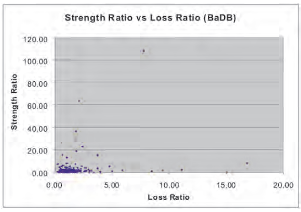 As can be seen, there are a few extreme outliers among these 243 data points. The most extreme, the Battle of Tippennuir (l Sep 1644), in which an English Royalist force under Montrose routed an attack by Scottish Covenanter militia, causing about 3,000 casualties to the Scots in exchange for a single (allegedly self-inflicted) casualty to the Royalists, was removed from the chart. This 3,000-to-1 loss ratio was deemed too great an outlier to be of value in the analysis.
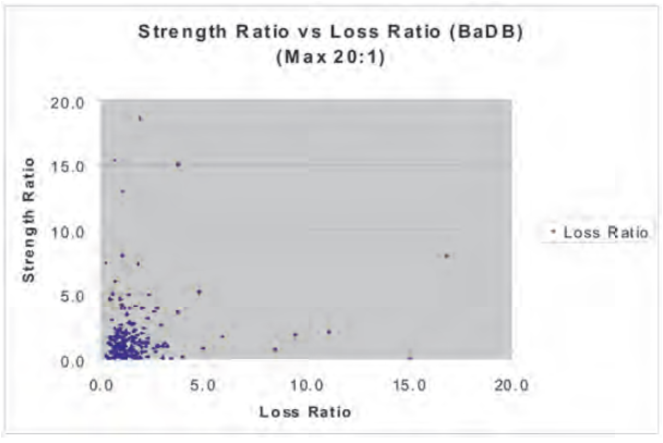 As it is, the vast majority of cases are clumped down into the corner of the graph with only a few scattered data points outside of that clumping. If one did try to establish some form of curvilinear relationship, one would end up drawing a hyperbola. It is worthwhile to look inside that clump of data to see what it shows. Therefore, we will look at the graph truncated so as to show only force ratios at or below 20-to-1 and exchange rations at or below 20-to-1.
 Again, the data remains clustered in one corner with the outlying data points again pointing to a hyperbola as the only real fitting curvilinear relationship. Let’s look at little deeper into the data by truncating the data on 6-to-1 for both force ratios and exchange ratios. As can be seen, if the RAND version of the 3-to-1 rule is correct, then the data should show at 3-to-1 force ratio a 3-to-1 casualty exchange ratio. There is only one data point that comes close to this out of the 243 points we examined.
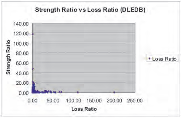 Even though this data covers from 1904 to 1991, with the vast majority of the data coming from engagements after 1940, one again sees the same pattern as with the data from 1600-1900. If there is a curvilinear relationship, it is again a hyperbola. As before, it is useful to look into the mass of data clustered into the corner by truncating the force and exchange ratios at 20-to-1. This produces the following:
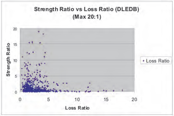 Again, one sees the data clustered in the corner, with any curvilinear relationship again being a hyperbola. A look at the data further truncated to a 10-to-1 force or exchange ratio does not yield anything more revealing.
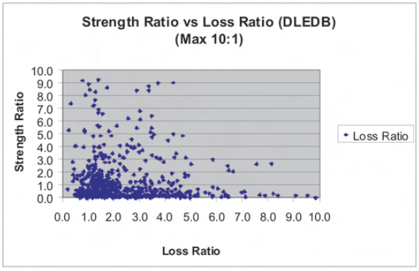 And, if this data is truncated to show only 5-to-1 force ratio and exchange ratios, one again sees:
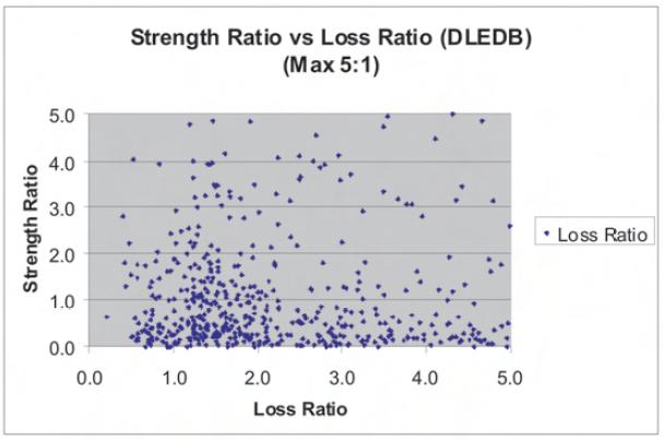 Again, this data appears to be mostly just noise, with no clear patterns here that support any of the three constructs. In the case of the RAND version of the 3-to-1 rule, there is again only one data point (out of 628) that is anywhere close to the crossover point (even fractional exchange rate) that RAND postulates. In fact, it almost looks like the data conspires to make sure it leaves a noticeable “hole” at that point. The other postulated versions of the 3-to-1 rules are also given no support in these charts.