The question of validating combat models—“To confirm or prove that the output or outputs of a model are consistent with the real-world functioning or operation of the process, procedure, or activity which the model is intended to represent or replicate”—as Trevor Dupuy put it, has taken up a lot of space on the TDI blog this year. What this discussion did not address is what an effort to validate a combat model actually looks like. This will be the first in a series of posts that will do exactly that.
Under the guidance of Christopher A. Lawrence, TDI undertook a battalion-level validation of Dupuy’s Tactical Numerical Deterministic Model (TNDM) in late 1996. This effort tested the model against 76 engagements from World War I, World War II, and the post-1945 world including Vietnam, the Arab-Israeli Wars, the Falklands War, Angola, Nicaragua, etc. It was probably one of the more independent and better-documented validations of a casualty estimation methodology that has ever been conducted to date, in that:
The data was independently assembled (assembled for other purposes before the validation) by a number of different historians.
There were no calibration runs or adjustments made to the model before the test.
The data included a wide range of material from different conflicts and times (from 1918 to 1983).
The validation runs were conducted independently (Susan Rich conducted the validation runs, while Christopher A. Lawrence evaluated them).
The results of the validation were fully published.
The people conducting the validation were independent, in the sense that:
a) there was no contract, management, or agency requesting the validation;
b) none of the validators had previously been involved in designing the model, and had only very limited experience in using it; and
c) the original model designer was not able to oversee or influence the validation. (Dupuy passed away in July 1995 and the validation was conducted in 1996 and 1997.)
The validation was not truly independent, as the model tested was a commercial product of TDI, and the person conducting the test was an employee of the Institute. On the other hand, this was an independent effort in the sense that the effort was employee-initiated and not requested or reviewed by the management of the Institute.
Descriptions and outcomes of this validation effort were first reported in The International TNDM Newsletter. Chris Lawrence also addressed validation of the TNDM in Chapter 19 of War by Numbers (2017).
As I stated in a previous post, I am not aware of any other major validation efforts done in the last 25 years other than what we have done. Still, there is one other effort that needs to be mentioned. This is described in a 2017 report: Using Combat Adjudication to Aid in Training for Campaign Planning.pdf
I gather this was work by J-7 of the Joint Staff to develop Joint Training Tools (JTT) using the Combat Adjudication Service (CAS) model. There are a few lines in the report that warm my heart:
“It [JTT] is based on and expanded from Dupuy’s Quantified Judgement Method of Analysis (QJMA) and Tactical Deterministic Model.”
“The CAS design used Dupuy’s data tables in whole or in part (e.g. terrain, weather, water obstacles, and advance rates).”
“Non-combat power variables describing the combat environment and other situational information are listed in Table 1, and are a subset of variables (Dupuy, 1985).”
“The authors would like to acknowledge COL Trevor N. Dupuy for getting Michael Robel interested in combat modeling in 1979.”
Now, there is a section labeled verification and validation. Let me quote from that:
CAS results have been “Face validated” against the following use cases:
The 3:1 rules. The rule of thumb postulating an attacking force must have at least three times the combat power of the defending force to be successful.
1st (US) Infantry Divison vers 26th (IQ) Infantry Division during Desert Storm
The Battle of 73 Easting: 2nd ACR versus elements of the Iraqi Republican Guards
3rd (US) Infantry Division’s first five days of combat during Operation Iraqi Freedom (OIF)
Each engagement is conducted with several different terrain and weather conditions, varying strength percentages and progresses from a ground only engagement to multi-service engagements to test the effect of CASP [Close Air Support] and interdiction on the ground campaign. Several shortcomings have been detected, but thus far ground and CASP match historical results. However, modeling of air interdiction could not be validated.
So, this is a face validation based upon three cases. This is more than what I have seen anyone else do in the last 25 years.
What we have listed in the previous articles is what we consider the six best databases to use for validation. The Ardennes Campaign Simulation Data Base (ACSDB) was used for a validation effort by CAA (Center for Army Analysis). The Kursk Data Base (KDB) was never used for a validation effort but was used, along with Ardennes, to test Lanchester equations (they failed).
The Battle of Britain Data Base to date has not been used for anything that we are aware of. As the program we were supporting was classified, then they may have done some work with it that we are not aware of, but I do not think that is the case.
Our three battles databases, the division-level data base, the battalion-level data base and the company-level data base, have all be used for validating our own TNDM (Tactical Numerical Deterministic Model). These efforts have been written up in our newsletters (here: http://www.dupuyinstitute.org/tdipub4.htm) and briefly discussed in Chapter 19 of War by Numbers. These are very good databases to use for validation of a combat model or testing a casualty estimation methodology. We have also used them for a number of other studies (Capture Rate, Urban Warfare, Lighter-Weight Armor, Situational Awareness, Casualty Estimation Methodologies, etc.). They are extremely useful tools analyzing the nature of conflict and how it impacts certain aspects. They are, of course, unique to The Dupuy Institute and for obvious business reasons, we do keep them close hold.
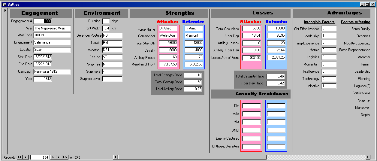
We do have a number of other database that have not been used as much. There is a list of 793 conflicts from 1898-1998 that we have yet to use for anything (the WACCO – Warfare, Armed Conflict and Contingency Operations database). There is the Campaign Data Base (CaDB) of 196 cases from 1904 to 1991, which was used for the Lighter Weight Armor study. There are three databases that are mostly made of cases from the original Land Warfare Data Base (LWDB) that did not fit into our division-level, battalion-level, and company-level data bases. They are the Large Action Data Base (LADB) of 55 cases from 1912-1973, the Small Action Data Base (SADB) of 5 cases and the Battles Data Base (BaDB) of 243 cases from 1600-1900. We have not used these three database for any studies, although the BaDB is used for analysis in War by Numbers.
Finally, there are three databases on insurgencies, interventions and peacekeeping operations that we have developed. This first was the Modern Contingency Operations Data Base (MCODB) that we developed to use for Bosnia estimate that we did for the Joint Staff in 1995. This is discussed in Appendix II of America’s Modern Wars. It then morphed into the Small Scale Contingency Operations (SSCO) database which we used for the Lighter Weight Army study. We then did the Iraq Casualty Estimate in 2004 and significant part of the SSCO database was then used to create the Modern Insurgency Spread Sheets (MISS). This is all discussed in some depth in my book America’s Modern Wars.
None of these, except the Campaign Data Base and the Battles Data Base (1600-1900), are good for use in a model validation effort. The use of the Campaign Data Base should be supplementary to validation by another database, much like we used it in the Lighter Weight Armor study.
Now, there have been three other major historical validation efforts done that we were not involved in. I will discuss their supporting data on my next post on this subject.
SMEs….is a truly odd sounding acronym that means Subject Matter Experts. They talk about it extensively in their article, and this I have no problem with. I do want to make three points related to that:
A SME is not a substitution for validation.
In some respects, the QJM (Quantified Judgment Model) is a quantified and validated SME.
How do you know that the SME is right?
If you can substitute a SME for a proper validation effort, then perhaps you could just substitute the SME for the model. This would save time and money. If your SME is knowledgable enough to sprinkle holy water on the model and bless its results, why not just skip the model and ask the SME. We could certainly simplify and speed up analysis by removing the models and just asking our favorite SME. The weaknesses of this approach are obvious.
Then there is Trevor N. Dupuy’s Quantified Judgment Model (QJM) and Quantified Judgment Method of Analysis (QJMA). This is, in some respects, a SME quantified. Actually it was a board of SMEs, who working with a series of historical studies (the list of studies starts here: http://www.dupuyinstitute.org/tdipubs.htm ). These SMEs developed a set of values for different situations, and then insert them into a model. They then validated the model to historical data (also known as real-world combat data). While the QJM has come under considerable criticism from elements of the Operations Research community…..if you are using SMEs, then in fact, you are using something akin, but less rigorous, than Trevor Dupuy’s Quantified Judgment Method of Analysis.
This last point, how do we know that the SME is right, is significant. How do you test your SMEs to ensure that what they are saying is correct? Another SME, a board of SMEs? Maybe a BOGSAT? Can you validate SMEs? There are limits to SME’s. In the end, you need a validated model.
More on the QJM/TNDM Italian Battles by Richard C. Anderson, Jr.
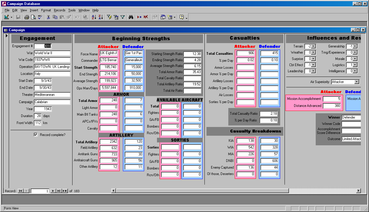
In regard to Niklas Zetterling’s article and Christopher Lawrence’s response (Newsletter Volume 1, Number 6) [and Christopher Lawrence’s 2018 addendum] I would like to add a few observations of my own. Recently I have had occasion to revisit the Allied and German records for Italy in general and for the Battle of Salerno in particular. What I found is relevant in both an analytical and an historical sense.
The Salerno Order of Battle
The first and most evident observation that I was able to make of the Allied and German Order of Battle for the Salerno engagements was that it was incorrect. The following observations all relate to the table found on page 25 of Volume 1, Number 6.
The divisional totals are misleading. The U.S. had one infantry division (the 36th) and two-thirds of a second (the 45th, minus the 180th RCT [Regimental Combat Team] and one battalion of the 157th Infantry) available during the major stages of the battle (9-15 September 1943). The 82nd Airborne Division was represented solely by elements of two parachute infantry regiments that were dropped as emergency reinforcements on 13-14 September. The British 7th Armored Division did not begin to arrive until 15-16 September and was not fully closed in the beachhead until 18-19 September.
The German situation was more complicated. Only a single panzer division, the 16th, under the command of the LXXVI Panzer Corps was present on 9 September. On 10 September elements of the Hermann Goring Parachute Panzer Division, with elements of the 15th Panzergrenadier Division under tactical command, began arriving from the vicinity of Naples. Major elements of the Herman Goring Division (with its subordinated elements of the 15th Panzergrenadier Division) were in place and had relieved elements of the 16th Panzer Division opposing the British beaches by 11 September. At the same time the 29th Panzergrenandier Division began arriving from Calabria and took up positions opposite the U.S. 36th Divisions in and south of Altavilla, again relieving elements of the 16th Panzer Division. By 11-12 September the German forces in the northern sector of the beachhead were under the command of the XIV Panzer Corps (Herman Goring Division (-), elements of the 15th Panzergrenadier Division and elements of the 3rd Panzergrenadier Division), while the LXXVI Panzer Corps commanded the 16th Panzer Division, 29th Panzergrenadier Division, and elements of the 26th Panzer Division. Unfortunately for the Germans the 16th Panzer Division’s zone was split by the boundary between the XIV and LXXVI Corps, both of whom appear to have had operational control over different elements of the division. Needless to say, the German command and control problems in this action were tremendous.[1]
The artillery totals given in the table are almost inexplicable. The numbers of SP [self-propelled] 75mm howitzers is a bit fuzzy, inasmuch as this was a non-standardized weapon on a half-track chassis. It was allocated to the infantry regimental cannon company (6 tubes) and was also issued to tank and tank destroyer battalions as a stopgap until purpose-designed systems could be brought into production. The 105mm SP was also present on a half-track chassis in the regimental cannon company (2 tubes) and on a full-track chassis in the armored field artillery battalion (18 tubes). The towed 105mm artillery was present in the five field artillery battalions present of the 36th and 45th divisions and in a single non-divisional battalion assigned to the VI Corps. The 155mm howitzers were only present in the two divisional field artillery battalions, the general support artillery assigned to the VI Corps, the 36th Field Artillery Regiment, did not arrive until 16 September. No 155mm gun battalions landed in Italy until October 1943. The U.S. artillery figures should approximately be as follows:
75mm Howitzer (SP)
2 per infantry battalion
28
6 per tank battalion
12
Total
40
105mm Howitzer (SP)
2 per infantry regiment
10
1 armored FA battalion[2]
18
5 divisional FA battalions
60
1 non-divisional FA battalion
12
Total
100
155mm Howitzer
2 divisional FA battalions
24
3″ Tank Destroyer
3 battalions
108
Thus, the U.S. artillery strength is approximately 272 versus 525 as given in the chart.
The British artillery figures are also suspect. Each of the British divisions present, the 46th and 56th, had three regiments (battalions in U.S. parlance) of 25-pounder gun-howitzers for a total of 72 per division. There is no evidence of the presence of the British 3-inch howitzer, except possibly on a tank chassis in the support tank role attached to the tank troop headquarters of the armor regiment (battalion) attached to the X Corps (possibly 8 tubes). The X Corps had a single medium regiment (battalion) attached with either 4.5 inch guns or 5.5 inch gun-howitzers or a mixture of the two (16 tubes). The British did not have any 7.2 inch howitzers or 155mm guns at Salerno. I do not know where the figure for British 75mm howitzers is from, although it is possible that some may have been present with the corps armored car regiment.
Thus the British artillery strength is approximately 168 versus 321 as given in the chart.
The German artillery types are highly suspect. As Niklas Zetterling deduced, there was no German corps or army artillery present at Salemo. Neither the XIV or LXXVI Corps had Heeres (army) artillery attached. The two battalions of the 7lst Nebelwerfer regiment and one battery of 170mm guns (previously attached to the 15th Panzergrenadier Division) were all out of action, refurbishing and replenishing equipment in the vicinity of Naples. However, U.S. intelligence sources located 42 Italian coastal gun positions, including three 149mm (not 132mm) railway guns defending the beaches. These positions were taken over by German personnel on the night before the invasion. That they fired at all in the circumstances is a comment on the professionalism of the German Army. The remaining German artillery available was with the divisional elements that arrived to defend against the invasion forces. The following artillery strengths are known for the German forces at Salerno:
501st Army Flak Battalion (probably 20mm and 37mm AA only)
I/49th Flak Battalion (probably 8 88mm AA guns)
Thus, German artillery strength is about 342 tubes versus 394 as given in the chart.[3]
Armor strengths are equally suspect for both the Allied and German forces. It should be noted however, that the original QJM database considered wheeled armored cars to be the equivalent of a light tank.
Only two U.S. armor battalions were assigned to the initial invasion force, with a total of 108 medium and 34 light tanks. The British X Corps had a single armor regiment (battalion) assigned with approximately 67 medium and 10 light tanks. Thus, the Allies had some 175 medium tanks versus 488 as given in the chart and 44 light tanks versus 236 (including an unknown number of armored cars) as given in the chart.
German armor strength was as follows (operational/in repair as of the date given):
16th Panzer Division (8 September):
7/0 Panzer III flamethrower tanks
12/0 Panzer IV short
86/6 Panzer IV long
37/3 assault guns
29th Panzergrenadier Division (1 September):
32/5 assault guns
17/4 SP antitank
3/0 Panzer III
26th Panzer Division (5 September):
11/? assault guns
10/? Panzer III
Herman Goering Parachute Panzer Division (7 September):
5/? Panzer IV short
11/? Panzer IV long
5/? Panzer III long
1/? Panzer III 75mm
21/? assault guns
3/? SP antitank
15th Panzergrenadier Division (8 September):
6/? Panzer IV long
18/? assault guns
Total 285/18 medium tanks, SP anti-tank, and assault guns. This number actually agrees very well with the 290 medium tanks given in the chart. I have not looked closely at the number of German armored cars but suspect that it is fairly close to that given in the charts.
In general it appears that the original QJM Database got the numbers of major items of equipment right for the Germans, even if it flubbed on the details. On the other hand, the numbers and details are highly suspect for the Allied major items of equipment. Just as a first order “guestimate” I would say that this probably reduces the German CEV to some extent; however, missing from the formula is the Allied naval gunfire support which, although negligible in impact in the initial stages of the battle, had a strong influence on the later stages of the battle.
Hopefully, with a little more research and time, we will be able to go back and revalidate these engagements. In the meantime I hope that this has clarified some of the questions raised about the Italian QJM Database.
NOTES
[1] Exacerbating the German command and control problems was the fact that the Tenth Army, which was in overall command of the XIV Panzer Corps and LXXVI Panzer Corps, had only been in existence for about six weeks. The army’s signal regiment was only partly organized and its quartermaster services were almost nonexistent.
[2] Arrived 13 September, 1 battery in action 13-15 September.
[3] However, the number given for the 29th Panzergrenadier Division appears to be suspiciously high and is not well defined. Hopefully further research may clarify the status of this division.
Shawn likes to post up on the blog old articles from The International TNDM Newsletter. The previous blog post was one such article I wrote in 1997 (he posted it under my name…although he put together the post). This is the first time I have read it since say….1997. A few comments:
In fact, we did go back in systematically review and correct all the Italian engagements. This was primarily done by Richard Anderson from German records and UK records. All the UK engagements were revised as were many of the other Italian Campaign records. In fact, we ended up revising at least half of the WWII engagements in the Land Warfare Data Base (LWDB).
We did greatly expand our collection of data, to over 1,200 engagements, including 752 in a division-level engagement database. Basically we doubled the size of the database (and placed it in Access).
Using this more powerful data collection, I then re-shot the analysis of combat effectiveness. I did not use any modeling structure, but simply just used basic statistics. This effort again showed a performance difference in combat in Italy between the Germans, the Americans and the British. This is discussed in War by Numbers, pages 19-31.
We did actually re-validate the TNDM. The results of this validation are published in War by Numbers, pages 299-324. They were separately validated at corps-level (WWII), division-level (WWII) and at Battalion-level (WWI, WWII and post-WWII).
War by Numbers also includes a detailed discussion of differences in casualty reporting between nations (pages 202-205) and between services (pages 193-202).
We have never done an analysis of the value of terrain using our larger more robust databases, although this is on my short-list of things to do. This is expected to be part of War by Numbers II, if I get around to writing it.
We have done no significant re-design of the TNDM.
Anyhow, that is some of what we have been doing in the intervening 20 years since I wrote that article.
Response to Niklas Zetterling’s Article by Christopher A. Lawrence
Mr. Zetterling is currently a professor at the Swedish War College and previously worked at the Swedish National Defense Research Establishment. As I have been having an ongoing dialogue with Prof. Zetterling on the Battle of Kursk, I have had the opportunity to witness his approach to researching historical data and the depth of research. I would recommend that all of our readers take a look at his recent article in the Journal of Slavic Military Studies entitled “Loss Rates on the Eastern Front during World War II.” Mr. Zetterling does his German research directly from the Captured German Military Records by purchasing the rolls of microfilm from the US National Archives. He is using the same German data sources that we are. Let me attempt to address his comments section by section:
The Database on Italy 1943-44:
Unfortunately, the Italian combat data was one of the early HERO research projects, with the results first published in 1971. I do not know who worked on it nor the specifics of how it was done. There are references to the Captured German Records, but significantly, they only reference division files for these battles. While I have not had the time to review Prof. Zetterling‘s review of the original research. I do know that some of our researchers have complained about parts of the Italian data. From what I’ve seen, it looks like the original HERO researchers didn’t look into the Corps and Army files, and assumed what the attached Corps artillery strengths were. Sloppy research is embarrassing, although it does occur, especially when working under severe financial constraints (for example, our Battalion-level Operations Database). If the research is sloppy or hurried, or done from secondary sources, then hopefully the errors are random, and will effectively counterbalance each other, and not change the results of the analysis. If the errors are all in one direction, then this will produce a biased result.
I have no basis to believe that Prof. Zetterling’s criticism is wrong, and do have many reasons to believe that it is correct. Until l can take the time to go through the Corps and Army files, I intend to operate under the assumption that Prof. Zetterling’s corrections are good. At some point I will need to go back through the Italian Campaign data and correct it and update the Land Warfare Database. I did compare Prof. Zetterling‘s list of battles with what was declared to be the forces involved in the battle (according to the Combat Data Subscription Service) and they show the following attached artillery:
It is clear that the battles were based on the assumption that here was Corps-level German artillery. A strength comparison between the two sides is displayed in the chart on the next page.
The Result Formula:
CEV is calculated from three factors. Therefore a consistent 20% error in casualties will result in something less than a 20% error in CEV. The mission effectiveness factor is indeed very “fuzzy,” and these is simply no systematic method or guidance in its application. Sometimes, it is not based upon the assigned mission of the unit, but its perceived mission based upon the analyst’s interpretation. But, while l have the same problems with the mission accomplishment scores as Mr. Zetterling, I do not have a good replacement. Considering the nature of warfare, I would hate to create CEVs without it. Of course, Trevor Dupuy was experimenting with creating CEVs just from casualty effectiveness, and by averaging his two CEV scores (CEVt and CEVI) he heavily weighted the CEV calculation for the TNDM towards measuring primarily casualty effectiveness (see the article in issue 5 of the Newsletter, “Numerical Adjustment of CEV Results: Averages and Means“). At this point, I would like to produce a new, single formula for CEV to replace the current two and its averaging methodology. I am open to suggestions for this.
Supply Situation:
The different ammunition usage rate of the German and US Armies is one of the reasons why adding a logistics module is high on my list of model corrections. This was discussed in Issue 2 of the Newsletter, “Developing a Logistics Model for the TNDM.” As Mr. Zetterling points out, “It is unlikely that an increase in artillery ammunition expenditure will result in a proportional increase in combat power. Rather it is more likely that there is some kind of diminished return with increased expenditure.” This parallels what l expressed in point 12 of that article: “It is suspected that this increase [in OLIs] will not be linear.”
The CEV does include “logistics.” So in effect, if one had a good logistics module, the difference in logistics would be accounted for, and the Germans (after logistics is taken into account) may indeed have a higher CEV.
General Problems with Non-Divisional Units Tooth-to-Tail Ratio
Point taken. The engagements used to test the TNDM have been gathered over a period of over 25 years, by different researchers and controlled by different management. What is counted when and where does change from one group of engagements to the next. While l do think this has not had a significant result on the model outcomes, it is “sloppy” and needs to be addressed.
The Effects of Defensive Posture
This is a very good point. If the budget was available, my first step in “redesigning” the TNDM would be to try to measure the effects of terrain on combat through the use of a large LWDB-type database and regression analysis. I have always felt that with enough engagements, one could produce reliable values for these figures based upon something other than judgement. Prof. Zetterling’s proposed methodology is also a good approach, easier to do, and more likely to get a conclusive result. I intend to add this to my list of model improvements.
Conclusions
There is one other problem with the Italian data that Prof. Zetterling did not address. This was that the Germans and the Allies had different reporting systems for casualties. Quite simply, the Germans did not report as casualties those people who were lightly wounded and treated and returned to duty from the divisional aid station. The United States and England did. This shows up when one compares the wounded to killed ratios of the various armies, with the Germans usually having in the range of 3 to 4 wounded for every one killed, while the allies tend to have 4 to 5 wounded for every one killed. Basically, when comparing the two reports, the Germans “undercount” their casualties by around 17 to 20%. Therefore, one probably needs to use a multiplier of 20 to 25% to match the two casualty systems. This was not taken into account in any the work HERO did.
Because Trevor Dupuy used three factors for measuring his CEV, this error certainly resulted in a slightly higher CEV for the Germans than should have been the case, but not a 20% increase. As Prof. Zetterling points out, the correction of the count of artillery pieces should result in a higher CEV than Col. Dupuy calculated. Finally, if Col. Dupuy overrated the value of defensive terrain, then this may result in the German CEV being slightly lower.
As you may have noted in my list of improvements (Issue 2, “Planned Improvements to the TNDM”), I did list “revalidating” to the QJM Database. [NOTE: a summary of the QJM/TNDM validation efforts can be found here.] As part of that revalidation process, we would need to review the data used in the validation data base first, account for the casualty differences in the reporting systems, and determine if the model indeed overrates the effect of terrain on defense.
Perhaps one of the most debated results of the TNDM (and its predecessors) is the conclusion that the German ground forces on average enjoyed a measurable qualitative superiority over its US and British opponents. This was largely the result of calculations on situations in Italy in 1943-44, even though further engagements have been added since the results were first presented. The calculated German superiority over the Red Army, despite the much smaller number of engagements, has not aroused as much opposition. Similarly, the calculated Israeli effectiveness superiority over its enemies seems to have surprised few.
However, there are objections to the calculations on the engagements in Italy 1943. These concern primarily the database, but there are also some questions to be raised against the way some of the calculations have been made, which may possibly have consequences for the TNDM.
Here it is suggested that the German CEV [combat effectiveness value] superiority was higher than originally calculated. There are a number of flaws in the original calculations, each of which will be discussed separately below. With the exception of one issue, all of them, if corrected, tend to give a higher German CEV.
The Database on Italy 1943-44
According to the database the German divisions had considerable fire support from GHQ artillery units. This is the only possible conclusion from the fact that several pieces of the types 15cm gun, 17cm gun, 21cm gun, and 15cm and 21cm Nebelwerfer are included in the data for individual engagements. These types of guns were almost exclusively confined to GHQ units. An example from the database are the three engagements Port of Salerno, Amphitheater, and Sele-Calore Corridor. These take place simultaneously (9-11 September 1943) with the German 16th Pz Div on the Axis side in all of them (no other division is included in the battles). Judging from the manpower figures, it seems to have been assumed that the division participated with one quarter of its strength in each of the two former battles and half its strength in the latter. According to the database, the number of guns were:
15cm gun
28
17cm gun
12
21cm gun
12
15cm NbW
27
21cm NbW
21
This would indicate that the 16th Pz Div was supported by the equivalent of more than five non-divisional artillery battalions. For the German army this is a suspiciously high number, usually there were rather something like one GHQ artillery battalion for each division, or even less. Research in the German Military Archives confirmed that the number of GHQ artillery units was far less than indicated in the HERO database. Among the useful documents found were a map showing the dispositions of 10th Army artillery units. This showed clearly that there was only one non-divisional artillery unit south of Rome at the time of the Salerno landings, the III/71 Nebelwerfer Battalion. Also the 557th Artillery Battalion (17cm gun) was present, it was included in the artillery regiment (33rd Artillery Regiment) of 15th Panzergrenadier Division during the second half of 1943. Thus the number of German artillery pieces in these engagements is exaggerated to an extent that cannot be considered insignificant. Since OLI values for artillery usually constitute a significant share of the total OLI of a force in the TNDM, errors in artillery strength cannot be dismissed easily.
While the example above is but one, further archival research has shown that the same kind of error occurs in all the engagements in September and October 1943. It has not been possible to check the engagements later during 1943, but a pattern can be recognized. The ratio between the numbers of various types of GHQ artillery pieces does not change much from battle to battle. It seems that when the database was developed, the researchers worked with the assumption that the German corps and army organizations had organic artillery, and this assumption may have been used as a “rule of thumb.” This is wrong, however; only artillery staffs, command and control units were included in the corps and army organizations, not firing units. Consequently we have a systematic error, which cannot be corrected without changing the contents of the database. It is worth emphasizing that we are discussing an exaggeration of German artillery strength of about 100%, which certainly is significant. Comparing the available archival records with the database also reveals errors in numbers of tanks and antitank guns, but these are much smaller than the errors in artillery strength. Again these errors do always inflate the German strength in those engagements l have been able to check against archival records. These errors tend to inflate German numerical strength, which of course affects CEV calculations. But there are further objections to the CEV calculations.
The Result Formula
The “result formula” weighs together three factors: casualties inflicted, distance advanced, and mission accomplishment. It seems that the first two do not raise many objections, even though the relative weight of them may always be subject to argumentation.
The third factor, mission accomplishment, is more dubious however. At first glance it may seem to be natural to include such a factor. Alter all, a combat unit is supposed to accomplish the missions given to it. However, whether a unit accomplishes its mission or not depends both on its own qualities as well as the realism of the mission assigned. Thus the mission accomplishment factor may reflect the qualities of the combat unit as well as the higher HQs and the general strategic situation. As an example, the Rapido crossing by the U.S. 36th Infantry Division can serve. The division did not accomplish its mission, but whether the mission was realistic, given the circumstances, is dubious. Similarly many German units did probably, in many situations, receive unrealistic missions, particularly during the last two years of the war (when most of the engagements in the database were fought). A more extreme example of situations in which unrealistic missions were given is the battle in Belorussia, June-July 1944, where German units were regularly given impossible missions. Possibly it is a general trend that the side which is fighting at a strategic disadvantage is more prone to give its combat units unrealistic missions.
On the other hand it is quite clear that the mission assigned may well affect both the casualty rates and advance rates. If, for example, the defender has a withdrawal mission, advance may become higher than if the mission was to defend resolutely. This must however not necessarily be handled by including a missions factor in a result formula.
I have made some tentative runs with the TNDM, testing with various CEV values to see which value produced an outcome in terms of casualties and ground gained as near as possible to the historical result. The results of these runs are very preliminary, but the tendency is that higher German CEVs produce more historical outcomes, particularly concerning combat.
Supply Situation
According to scattered information available in published literature, the U.S. artillery fired more shells per day per gun than did German artillery. In Normandy, US 155mm M1 howitzers fired 28.4 rounds per day during July, while August showed slightly lower consumption, 18 rounds per day. For the 105mm M2 howitzer the corresponding figures were 40.8 and 27.4. This can be compared to a German OKH study which, based on the experiences in Russia 1941-43, suggested that consumption of 105mm howitzer ammunition was about 13-22 rounds per gun per day, depending on the strength of the opposition encountered. For the 150mm howitzer the figures were 12-15.
While these figures should not be taken too seriously, as they are not from primary sources and they do also reflect the conditions in different theaters, they do at least indicate that it cannot be taken for granted that ammunition expenditure is proportional to the number of gun barrels. In fact there also exist further indications that Allied ammunition expenditure was greater than the German. Several German reports from Normandy indicate that they were astonished by the Allied ammunition expenditure.
It is unlikely that an increase in artillery ammunition expenditure will result in a proportional increase combat power. Rather it is more likely that there is some kind of diminished return with increased expenditure.
General Problems with Non-Divisional Units
A division usually (but not necessarily) includes various support services, such as maintenance, supply, and medical services. Non-divisional combat units have to a greater extent to rely on corps and army for such support. This makes it complicated to include such units, since when entering, for example, the manpower strength and truck strength in the TNDM, it is difficult to assess their contribution to the overall numbers.
Furthermore, the amount of such forces is not equal on the German and Allied sides. In general the Allied divisional slice was far greater than the German. In Normandy the US forces on 25 July 1944 had 812,000 men on the Continent, while the number of divisions was 18 (including the 5th Armored, which was in the process of landing on the 25th). This gives a divisional slice of 45,000 men. By comparison the German 7th Army mustered 16 divisions and 231,000 men on 1 June 1944, giving a slice of 14,437 men per division. The main explanation for the difference is the non-divisional combat units and the logistical organization to support them. In general, non-divisional combat units are composed of powerful, but supply-consuming, types like armor, artillery, antitank and antiaircraft. Thus their contribution to combat power and strain on the logistical apparatus is considerable. However I do not believe that the supporting units’ manpower and vehicles have been included in TNDM calculations.
There are however further problems with non-divisional units. While the whereabouts of tank and tank destroyer units can usually be established with sufficient certainty, artillery can be much harder to pin down to a specific division engagement. This is of course a greater problem when the geographical extent of a battle is small.
Tooth-to-Tail Ratio
Above was discussed the lack of support units in non-divisional combat units. One effect of this is to create a force with more OLI per man. This is the result of the unit‘s “tail” belonging to some other part of the military organization.
In the TNDM there is a mobility formula, which tends to favor units with many weapons and vehicles compared to the number of men. This became apparent when I was performing a great number of TNDM runs on engagements between Swedish brigades and Soviet regiments. The Soviet regiments usually contained rather few men, but still had many AFVs, artillery tubes, AT weapons, etc. The Mobility Formula in TNDM favors such units. However, I do not think this reflects any phenomenon in the real world. The Soviet penchant for lean combat units, with supply, maintenance, and other services provided by higher echelons, is not a more effective solution in general, but perhaps better suited to the particular constraints they were experiencing when forming units, training men, etc. In effect these services were existing in the Soviet army too, but formally not with the combat units.
This problem is to some extent reminiscent to how density is calculated (a problem discussed by Chris Lawrence in a recent issue of the Newsletter). It is comparatively easy to define the frontal limit of the deployment area of force, and it is relatively easy to define the lateral limits too. It is, however, much more difficult to say where the rear limit of a force is located.
When entering forces in the TNDM a rear limit is, perhaps unintentionally, drawn. But if the combat unit includes support units, the rear limit is pushed farther back compared to a force whose combat units are well separated from support units.
To what extent this affects the CEV calculations is unclear. Using the original database values, the German forces are perhaps given too high combat strength when the great number of GHQ artillery units is included. On the other hand, if the GHQ artillery units are not included, the opposite may be true.
The Effects of Defensive Posture
The posture factors are difficult to analyze, since they alone do not portray the advantages of defensive position. Such effects are also included in terrain factors.
It seems that the numerical values for these factors were assigned on the basis of professional judgement. However, when the QJM was developed, it seems that the developers did not assume the German CEV superiority. Rather, the German CEV superiority seems to have been discovered later. It is possible that the professional judgement was about as wrong on the issue of posture effects as they were on CEV. Since the British and American forces were predominantly on the offensive, while the Germans mainly defended themselves, a German CEV superiority may, at least partly, be hidden in two high effects for defensive posture.
When using corrected input data on the 20 situations in Italy September-October 1943, there is a tendency that the German CEV is higher when they attack. Such a tendency is also discernible in the engagements presented in Hitler’s Last Gamble. Appendix H, even though the number of engagements in the latter case is very small.
As it stands now this is not really more than a hypothesis, since it will take an analysis of a greater number of engagements to confirm it. However, if such an analysis is done, it must be done using several sets of data. German and Allied attacks must be analyzed separately, and preferably the data would be separated further into sets for each relevant terrain type. Since the effects of the defensive posture are intertwined with terrain factors, it is very much possible that the factors may be correct for certain terrain types, while they are wrong for others. It may also be that the factors can be different for various opponents (due to differences in training, doctrine, etc.). It is also possible that the factors are different if the forces are predominantly composed of armor units or mainly of infantry.
One further problem with the effects of defensive position is that it is probably strongly affected by the density of forces. It is likely that the main effect of the density of forces is the inability to use effectively all the forces involved. Thus it may be that this factor will not influence the outcome except when the density is comparatively high. However, what can be regarded as “high” is probably much dependent on terrain, road net quality, and the cross-country mobility of the forces.
Conclusions
While the TNDM has been criticized here, it is also fitting to praise the model. The very fact that it can be criticized in this way is a testimony to its openness. In a sense a model is also a theory, and to use Popperian terminology, the TNDM is also very testable.
It should also be emphasized that the greatest errors are probably those in the database. As previously stated, I can only conclude safely that the data on the engagements in Italy in 1943 are wrong; later engagements have not yet been checked against archival documents. Overall the errors do not represent a dramatic change in the CEV values. Rather, the Germans seem to have (in Italy 1943) a superiority on the order of 1.4-1.5, compared to an original figure of 1.2-1.3.
During September and October 1943, almost all the German divisions in southern Italy were mechanized or parachute divisions. This may have contributed to a higher German CEV. Thus it is not certain that the conclusions arrived at here are valid for German forces in general, even though this factor should not be exaggerated, since many of the German divisions in Italy were either newly raised (e.g., 26th Panzer Division) or rebuilt after the Stalingrad disaster (16th Panzer Division plus 3rd and 29th Panzergrenadier Divisions) or the Tunisian debacle (15th Panzergrenadier Division).
My new book, with a release date of 1 August, is now available on Amazon.com for pre-order: War by Numbers (Amazon)
It is still listed at 498 pages, and I am pretty sure I only wrote 342. I will receive the proofs next month for review, so will have a chance to see how they got there. My Kursk book was over 2,500 pages in Microsoft Word, and we got it down to a mere 1,662 pages in print form. Not sure how this one is heading the other way.
Unlike the Kursk book, there will be a kindle version.
It is already available for pre-order from University of Nebraska Press here: War by Numbers (US)
It is available for pre-order in the UK through Casemate: War by Numbers (UK)
During the Cold War Sweden and Finland were two nations that were democratic and independent but were neutral and not part of NATO. Norway and Denmark were a part of NATO since 1949 and the three Baltic states (Lithuania, Latvia and Estonia) were part of the Soviet Union since 1940. Now the three Baltic states are part of NATO as of 2004 and Sweden and Finland are establishing ties to NATO.
Just a little demographics: the population of Scandinavia is around 27 million people, that is 5 million in Norway (which has a per capita income higher than the U.S.), 10 million in Sweden, 5.5 million in Finland, over 5.5 million in Denmark, plus Iceland and the Faroe Islands. The population of the three Baltic states is around 6 million people (and includes four major languages, including Russian). The population of Russia is 144 million (with 5 million in St. Petersburg and less than a million in the Kaliningrad Oblast).
We have sold the rights to use our combat model, the TNDM (Tactical Numerical Deterministic Model) to Sweden and Finland. We have never the rights to use the combat model to a NATO member.
 The question of validating combat models—“To confirm or prove that the output or outputs of a model are consistent with the real-world functioning or operation of the process, procedure, or activity which the model is intended to represent or replicate”—as Trevor Dupuy put it, has taken up a lot of space on the TDI blog this year. What this discussion did not address is what an effort to validate a combat model actually looks like. This will be the first in a series of posts that will do exactly that.