Category TNDM

Wargaming 101: The Bad Use of a Good Tool

Another William “Chip” Sayers article. He has done over a dozen postings to this blog. Some of his previous postings include:

Wargaming 101: A Tale of Two Forces | Mystics & Statistics (dupuyinstitute.org)

A story about planning for Desert Storm (1991) | Mystics & Statistics (dupuyinstitute.org)


Wargaming 101:  The Bad Use of a Good Tool

In the mid to late 1980s, an office tasked with analysis and support concerning our NATO allies used Col. Dupuy’s Quantified Judgement Model (the predecessor of the TNDM) in analyzing the probable performance of NATO forces in the event of a conventional war in Europe. Why their counterpart for Soviet/Warsaw Pact countries, did not buy the QJM nor, apparently, participate in this analysis is unknown. The NATO office set out to do a series of analytical papers on the various NATO corps areas, presumably producing a study for each. Only two studies were published, one for each of two of the Corps that were considered NATO’s weakest. 

To understand how this project was conceived and designed, one needs to be familiar with NATO’s basic force structure for the Cold War. NATO’s Central Region was divided into eight national corps “slices.” The British, Dutch and Belgians each contributed one corps while the US provided two (plus a third that could rapidly deploy manpower from CONUS to fall in on prepositioned equipment) and the Germans three. Stacked together, they made up what was commonly referred to as the “layer cake” by those who saw fundamental weakness in this scheme. 

By assigning each nation a front-line area to defend, all of NATO would be involved from the outset, with no room for political maneuver — less resolute nations would be locked in from the start of the conflict. However, this meant that certain corps sectors were defended by suspect armies, creating opportunities for Soviet forces to breakthrough NATO’s main line of resistance and romp through their vulnerable and lucrative rear areas. NATO partially compensated by narrowing some of the weaker corps’ sectors and assigning more frontage to the stronger corps. Nevertheless, many believed this scheme of defense was more about politics and less about warfighting.

From North to South, NATO’s Northern Army Group (NORTHAG) consisted of I Netherlands (NE) Corps, I German (GE) Corps, I British (UK) Corps and I Belgian (BE) Corps. Immediately South of NORTHAG was NATO’s Central Army Group (CENTAG), made up of III GE Corps, US Seventh Army (V US Corps and VII US Corps) and II GE Corps.

The first thing one might notice about this arrangement of national corps sectors is that they vaguely look like cylinders of an in-line engine and would take little imagination to envision the Warsaw Pact forces as pistons attempting to push through those cylinders. In fact, a lot of 1980s Pentagon-type wargaming was done based on this idea. Of course, there are a couple of problems inherent to this concept. First, the Soviets knew there would be boundaries between the NATO corps, and that those boundaries would be natural weak points in the defensive scheme. How does one replicate that in a piston-based model? Second, it does not allow for maneuver, particularly across corps boundaries, but also within the “cylinder.” One rather expensive system by a beltway bandit contractor attempted to compensate in their piston-based model by using some mathematical modification, but this never proved convincing. Piston-based models were imminently tempting, but they were a trap that should never have been used. The first time I encountered one, I commented to a friend that I had better wargames in my closet at home, and they cost a whole lot less: $40, vice $1,000,000. I could have saved the Pentagon a lot of money on that one.

Unfortunately, the analysts in question fell for the piston trap. With apparently little or no input from their Soviet counterparts, they chose a relatively weak Soviet Combined Arms Army to act as an attacker, lined them up in the cylinder and sent them off in what was conceptually a simple frontal attack.

Feeding this rather simplistic scenario into the QJM gave results that were satisfying, but would have been suspect to analysts familiar with Soviet Army doctrine. In essence, the study’s analysts “found” that a weak NATO corps could successfully hold off a Soviet CAA and, by implication, a strong corps might be able to defeat or even successfully counterattack its Soviet assailant. A recent QJM run of this scenario resulted in an advance rate of only 2.7km per day — approximately 10% of Soviet planning norms. The second study had similar results, reinforcing their views. Both studies were beautifully done with color graphics and lavish detail. I was green with envy. My agency should have done one of these studies for each NATO corps, and they should have been done with much more understanding of how both sides would fight. It was a huge missed opportunity.

Unfortunately, these beautiful studies were foundationally flawed and would have misled had they gained traction. I don’t know why they failed to do that, whether it was patently obvious to Soviet analysts that the studies were wrong, whether no one believed in the QJM, or whether they were a tree falling in a forest with no one to hear. Most likely, they simply hit the street too late to be of interest, because the Warsaw Pact was crumbling and taking the Soviet threat to Europe off the board.

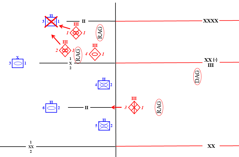
The studies’ analysts made several fundamental errors in setting up their scenarios.  First and foremost, they misjudged the threat they were working against. They posited that the weakest corps in NATO would face off against a weak Combined Arms Army with no reinforcement. Nothing could have been further from the truth. The Soviets knew NATO’s strengths and weaknesses — in some cases, apparently better than NATO itself — and had no intention of pitting weakness against weakness. Take a look at the following illustration, typical of the time and with at least a fair understanding of how the Soviets planned to go to war:

Note the thrust through Göttingen. Clearly, this is the main effort for the entire Western TVD (Theater of Military Operations). Rather than attack with a weak CAA, the Soviets would likely have thrown the full weight of their operation at the Schwerpunkt of the weak NATO corps. Not only would the strongest Soviet CAA made the attack, it would have had the assistance of second echelon artillery brigades whose parent armies were yet committed, their organic air support, and the lion’s share of Front supporting assets, as well — a very formidable force, indeed.

A second major mistake the studies’ analysts made was assuming that the Soviet thrust would have respected NATO corps boundaries. Take another look at the illustration, above. The main thrust is clearly divided between two armies. It was typical of Soviet battle planning that two adjacent armies would plan their breakthroughs to be side-by-side to take advantage of the potential for sharing supporting assets, to double the size of the breakthrough, and to add to the enemy’s confusion and dislocation by presenting a perplexing attack exploiting seams between defending corps. These two mistakes are why I surmise that Soviet analysts didn’t participate in the study. Surely, they would have corrected these errors.

These were problems with the scenario, but the modeling they did was fatally flawed in itself. If one is examining an operation at a particular level, one must use sub elements of that level to do a proper exploration. To simply feed the model two sides and press “start” is to believe in magic — that the model is able to sort out how the units would interact. By simply dumping the two sides into the model and pressing “start,” they were modeling a simple frontal attack circa 1915. To get legitimate results, the analysts must contribute more than this. 

The QJM was scaled to division/day operations, which means it works best if the maneuver elements are divisions. It works well with brigades/regiments and even down to the battalion and company levels. If the analysts wanted to explore the operations of a corps, they should, at a minimum, have laid out a division-level defense. Better yet, they should have taken it down to the brigade-level to account for nuance. Certainly, the model would have had no problem doing so and the results obtained would have been far more believable. Yet they did their simulation at the corps level, with no maneuver attempted. It’s no wonder they got such desultory results. Unfortunately, the analysts didn’t understand this.

So, how should the QJM have been used to better shed light on the reality of the situation? Clearly, the studies’ analysts needed a better order of battle for the Soviet side. Soviet analysts should have provided that for them, and it assuredly would have been more formidable than what they came up on their own. Further, they needed Soviet experts to set up a better attack for them. It should have included a mix of low-combat power attacks designed to fix enemy forces in place over wide frontages, and high-combat power attacks over a limited frontage to achieve the actual penetration of enemy defenses. Finally, they should have set up a detailed defense. Generically, it would have looked something like this:

A generic NATO corps of two mechanized divisions and a mechanized brigade in a “2 up, 1 back” defensive posture.  

In terms of raw combat power, the CAA with no reinforcement had a 2:1 advantage of the defending corps. Modifying the defenders for posture and terrain and other operational factors drove this down to a 1.6:1 advantage.

Our NATO corps defended approximately 40km of frontage divided between two mechanized divisions. One brigade of the northernmost division defended relatively open ground and was the target of the Soviet breakthrough attack. The second brigade of that division and the entire southern division occupied defensive positions on rougher ground and would therefore be subject to economy of force fixing attacks. The two divisions together had eight front-line battalions in the main line of resistance, each on a defensive frontage of 5km — a fairly comfortable force-to-space ratio. Unfortunately for NATO, the Soviet’s breakthrough frontage norms could be compressed to as little as 4km for a division with two regiments leading. In this case, that could mean a single defending battalion would receive the full weight of an entire attacking division, plus its attached fire support means. This might be one thing with a modern, well-equipped, well-trained, and well-supported corps. However, the NATO corps in question was none of these things.

The Soviet Army immediately to the north of our CAA had a more challenging enemy to overcome, so it chose to make its breakthrough attack through the northernmost battalion sector of our weak NATO corps. By aligning these two attacks on their common border, the Soviets ended up with a breakthrough zone of 10km and were able to share resources and targets.

A strictly numerical accounting of the breakthrough would show two defending companies of APC-mounted infantry at the line of contact with a third in depth, behind them. This array would be hit with a short but supremely violent “hurricane” barrage of over 400 artillery tubes and rocket launchers. This would be achieved by using the division’s organic assets (144 systems), plus the assets of an unengaged second-echelon division (144 systems), plus the CAA’s organic artillery brigade (72 systems — an unengaged a second-echelon army’s artillery brigade could provide support to another attacking division), plus assets from the CAA’s MRL regiment (54 systems).

From the unclassified DIA report, DDB-1130-8-82 Soviet Front Fire Support 15Dec81.

400 tubes firing at an average rate of five rounds a minute for 20 minutes would equate to roughly 40,000 rounds at a rate of 34 rounds per second on the positions of a single defending battalion. According to Soviet fire support norms, this is sufficient to completely suppress 12 company positions — 25% in excess of requirements for this attack. And this is without counting Army and Frontal Aviation airstrikes that would be allocated to any breakthrough attempt.

What are the practical effects of such a fire-strike? According to Soviet norms, ‘’A suppressed target has suffered damage sufficient to cause it to temporarily lose its combat effectiveness, or to be restricted in its ability to maneuver or effect command and control. Expressed mathematically, an area target is considered to be “suppressed” when it is highly probable (90 percent) that no less than 25 to 30 percent of the sub-elements of the target or 25 to 30 percent of the target’s area has suffered serious damage.” Put simply, the targeted battalion can be expected to lose a quarter of its combat power before the leading tank and motorized-rifle units engage. Further, many units will reach their breakpoint after 25% losses in such a short period of time, particularly those with lower levels of readiness and morale. Graphically, this can be illustrated in the following manner:

The CAA’s Chief of Rocket Troops and Artillery (CRTA) devises a 20-minute suppressive fire-strike in the breakthrough sector of the targeted NATO corps.  Meanwhile, the adjacent CAA is preparing its breakthrough attack in a similar manner.

Before NATO forces can commit reinforcements, the adjacent CAAs have blown a hole 10km wide in the NATO defenses, with little hope of checking the momentum of the deluge..

The breakthrough attack in the 2nd battalion/1st Mech sector is made at more than a 7:1 superiority yielding an advance rate of 24km per day, 16% casualties and a loss of 3/4s of the defenders combat power, effectively eliminating the battalion from the NATO order of battle. In the fixing attack immediately to the south, the slightly reinforced MRR is unable to make any ground, but neither would the NATO mechanized brigade, should it attempt a counterattack. Essentially, these two forces are locked together in stalemate, which is all that the Soviets needed for this attack to achieve its goals. The Soviet’s second MRD would have similar results against the NATO second mechanized division to the south.

The defending armored battalion is hit by four regiments (the two from the adjacent CAA not shown) and quickly overrun.

It is easy to see that the 1st Brigade’s 3rd Armored Battalion would be quickly overrun by the four-regiment freight train barreling down the line at it, but could the 1st Mech Division’s 3rd Armored Brigade — the Soviet Division’s subsequent objective — do better? With the Division’s 2nd echelon Tank Regiment committed, the attacker achieves a 2.3:1 superiority, which yields a 6.7km per day rate of advance and inflicts a 38% loss in combat power on the defender. That’s not a satisfactory rate of advance, but it is quite sufficient to keep the defending brigade from interfering with the commitment of the CAA’s second echelon, a tank division, for which the NATO corps has no answer.

While the 1st MRD pushes the NATO Corps’ armored brigade out of the way, the CAA’s second echelon tank division is committed into NORTHAG’s rear.

The European analysts predicted that there would be no penetration of the NATO corps’ defensive line. However, it took very little imagination to pass an entire tank division through while destroying a significant amount of the defender’s combat power. The QJM supported both outcomes, but it is not difficult to see that the details matter. The QJM/TNDM models are very good, but they are only as good as the user input. Flawed input may come from poor intelligence (in contemporary analysis) or from incomplete or inaccurate historical data (in the case of historical analysis). As we saw in this case, it can also come from a poor understanding of how one or both sides will fight.

Drone Survivability

On 30 June, we posted a guest post from William (Chip) Sayers on Scoring the KF51 Panther and the Future of the MBT | Mystics & Statistics (dupuyinstitute.org). The article generated some discussion on the blog which he partially responded to, but he felt the need to assemble a proper response. This is included below:

KF51 Panther. Image Credit: Industry Handout.

——–William (Chip) Sayers———————-

After submitting my post last week, we had a little internal debate among ourselves concerning the viability of drones and their ability to displace the MBT as the apex predator of the battlespace. What follows is a rather lengthy expansion of my reply to my colleagues.

I have written quite a bit on other fora about our over estimation of what drones – particularly of the Medium Altitude/Long Endurance (MALE) and High-Altitude/Long-Endurance (HALE) varieties – are capable of doing in the battlespace. I believe them to be virtually unsurvivable in a modern air defense environment — though I may have to up their chances a bit, given that they Russians have not, so far, swept them from the skies of Ukraine.  

The Turkish TB-2 is almost an exact analog of our MQ-1 Predator, and our experience with that system has been very instructive.  Iranians and Saddam-era Iraqis have been able to shoot them down, despite their general incompetence. The target drones we use to train fighter pilots and air defense crews in live-fire weapons employment exercises are far more challenging targets. This is because the Predator and other similar drones have an exceedingly limited ability to see the world around them. The pilot flies using a fixed nose camera with what is commonly referred to as a “soda-straw” view forward. The enemy interceptor (be it a fighter or a SAM) has to literally fly directly in front of the drone for the pilot to see it. The weapon systems operator is a bit better off as his camera is mounted in a turret, but again, it has to be pointed to within a few degrees of the interceptor, and coordination between the two “aircrew” in such a scenario is problematic, at best. In practice, however, they rarely even perceive when they are under attack and can’t do anything about it if they do: large, light-structured, straight-wing drones are not designed for maneuverability and have very little chance of survival, once targeted. Watching drone footage of an armed fighter-interceptor flashing by, and then, after a few seconds, seeing the video feed turn to static gives one a supreme feeling of helplessness.

Worse, drone accident rates are high and often due to things a pilot could avoid, if he were on board. Flying from a remote ground station just does not give a pilot the feel and visual scan that he would otherwise have. In the 1990s, we lost the entire Predator fleet over former-Yugoslavia, mostly to icing that could easily have been avoided if the aircraft were manned. An onboard pilot might have picked up the subtle clues through his controls and might have seen the ice beginning to form. With such information, he might have been able to simply change his altitude and continue the mission, or abort and save a valuable platform. While drone accident rates have come down from the disastrous levels of the 1990s, they remain at least twice those of the worst of USAF fighters.

Taken together, these drones are less survivable in a combat situation and succumb to accidents at a high rate making them much less effective and much more expensive than people generally believe. 
 
On the other hand, the Switchblade and the HERO-120 are in a completely different category. They are both significantly smaller than a MALE (length 4.25 vs 21 feet, wingspan of ~4 vs 39 feet and a weight of 50 vs 1,500lbs) and they use electric motors, making them acoustically undetectable and difficult to find with IR sensors. Shooting down one of these things flying just above the treetops isn’t impossible – if you see it – but it will be significantly more difficult than shooting down a MALE flying fat, dumb and happy at 15,000 feet. 

Nevertheless, these small drones are not without their vulnerabilities. They are already threatened by Counter-Rocket and Mortar (C-RAM) systems, designed to shoot down individual indirect fire rounds fired at fixed targets. These systems already acquire and track small-signature targets, so kamikaze drones won’t present the challenge they do to more traditional air defense systems. The main drawback that will keep C-RAM systems in check is their expense and limited mobility. More menacing in the not-too-distant future will be ground-based Laser air defense weapons when they come into operational use. A larger aircraft can take a hit in the fuselage or wing, and as long as it doesn’t contain a vital system at that point, it may be able to shrug off the hit. Not so with mini-drones where their small size will work against them as a hit anywhere will not require much dwell time to do catastrophic damage. Virtually any part of the drone’s volume will contain vital systems. So, look for kamikaze drones as the first target of air defense Lasers when they finally come online.

Some have talked of an anti-drone role for systems such as the Switchblade 300. Presumably, this would involve acquiring the target drone, flying a collision course and detonating the warhead within lethal range of the enemy craft. This is no easy feat with no dedicated acquisition and tracking means and working in three dimensions. This might work better against a less maneuverable, large target like a HALE or MALE UAS, but altitude and airspeed limitations work against the mini-drones here. Generally speaking, the smaller the drone, the less power and thus speed and altitude capability are available.

The final threat to the kamikaze drone is the most readily available and, perhaps, the most effective: jamming. These drones use radio signals to communicate with their operators and have little capability to operate autonomously, other than to cruise to a designated waypoint. If the link between drone and operator is broken, the drone is effectively neutralized. It is possible to give these drones an autonomous target recognition capability, but this takes sensors, computing capacity and electrical power, all of which require space in an already packed airframe. It is also has somewhat less than ideal reliability and represents a tangible threat to friendly forces.

Historically, whenever electro-magnetic jamming has come into play, it has always become a game of measure vs. countermeasure. Once started, the cycle cannot be relied on to stabilize in favor of one side or the other for very long. The implication is that kamikaze drones will have their moments of relative effectiveness, but they are unlikely to be swept from the sky by any single solution and thus will be an endemic feature of the battlespace for the foreseeable future.


Scoring the KF51 Panther and the Future of the MBT

KF51 Panther. Image Credit: Industry Handout.

Another William (Chip) Sayers post. This is his fifth post here. He will be presenting at our Historical Analysis conference: Who’s Who at HAAC – part 1 | Mystics & Statistics (dupuyinstitute.org).

———————–William (Chip) Sayers——————

Scoring the KF51 Panther and the Future of the MBT


The German arms manufacturer Rheinmetall recently announced the rollout of their newest Main Battle Tank, the KF51 Panther. The new tank has captured the attention of the world largely because its main armament represents the first major improvement in that area in over 40 years, but also because — let’s be honest — the prospect of a new German Panther prowling the battlefields of Europe just sounds incredibly sexy.

Panther Ausf D number 435 of the 51st Panzer Battalion Kursk (source: World War Photos 2013-2022, contact: info(at)worldwarphptos.info).

While the Panther is not yet approved for large-scale production by the Bundeswehr — it is, in fact, an alternative to an ongoing Franco-German Leopard II/AMX-40 Le Clerc replacement program — the buzz created by the name alone may propel it to top of the list. Rheinmetall’s announcement make it clear that the major selling features center around its new 130mm gun and autoloader (reducing the crew size to three), integral HERO-120 reconnaissance/weapon UAS, a new, more powerful diesel power plant, an active protection system and integrated vehicle electronics.

When a major new weapons system like the Panther enters the scene, I immediately reach for my TNDM Operational Lethality Index (OLI) creation spreadsheet and see how it scores. First, because it may come in handy in future modeling, but also because going through the process and examining the outcome has a tendency to cut through my preconceptions and replace them with a more balanced perspective. So, I thought I was share my insights with this post.

In creating a score for a tank, the first thing one must do is define and score the weapons systems. This presents a couple of challenges in the case of the KF51. First, there is little publicly available data on the Rh-130 gun. It will obviously be more powerful than the Rh-120 on the Leopard II, but we need more specificity to create a reasonable score. By scouring everything available on the web, I found claims of an effective range of 4,000 meters. I could not find an exact number for muzzle velocity, but 2,000 m/sec seems to be within the range of most speculation and seems, if anything, comfortably conservative. These are the really important numbers, so the main gun looks reasonably accounted for.

However, another aspect of the Rh-130 is its autoloader. Rheinmetall apparently believes that handling 130mm rounds inside a turret is too difficult to be done efficiently by a human loader and has substituted a mechanical device that can load the gun more quickly and without tiring over time. The downside of the autoloader is its small “ready use” capacity of 20 rounds. The OLI of a gun is based on its hourly rate of fire, which means that barrel heating and wear, and human fatigue need to be accounted for — and, it must be said, such numbers are not easily found. Fortunately, graphs for rate of fire based on shell-size are provided if reliable information is unavailable. On the other hand, magazine capacity is not the primary determinator of rate of fire. The rules for building a gun score state that one should not consider logistics as a limitation. In other words, it is as though the gun is on the range with an unlimited amount of ammunition available. Thus, while limited magazine capacity may yield a negative modifier, it isn’t an absolute limiter.

More difficult to calculate is the HERO-120. Not only are hard numbers difficult to come by, the TNDM has difficulty coming to grips with this system. The HERO-120 can serve as a basic reconnaissance UAS, but the TNDM has no explicit reconnaissance function — the model assumes that a given force has its doctrinal recon means operating in a competent manner. If this isn’t the case for some reason, the penalty would be assessed as a decrement in that side’s Combat Effectiveness Value (troop quality) or a
CEV bonus to the opposing side.

There are several ways we can score the HERO-120: as an infantry weapon, an ATGM, an artillery weapon, or as an aircraft. There is no clear-cut answer to how its score it. The HERO-120 can be used as an anti-personnel/light-materiel weapon that could be considered a long-range mortar within the confines of the model. Scoring it this way, the HERO-120 has an impressive Operational Lethality Index (combat power score) of 792. This compares to an AKM assault rifle at .16, an M-2HB .50 cal heavy machinegun at 1.2, or an M-43 120mm mortar at an OLI of 145.

Scoring it as an ATGM yields an OLI of 257. This compares well with the Russian Konkurs (113), Kornet-E (175), US TOW-2B (136) and Javelin-C (246). This is primarily due to the HERO-120’s much greater range. Scored as an artillery system — much like an MRL rocket or SSM — the HERO-120 has an OLI of 782. This compares to the 227mm HIMARS MLRS at 338, or a Russian 9K720 Iskander SSM at 184. Compared to the basic HIMARS, HERO-120 has better range and is much more accurate. Its major advantages over the Iskander are its guidance system and its much smaller size that makes it handier to reload, giving it a higher volume of firepower.

The obvious course is to score it as a fixed-wing aircraft, but this is a bit trickier than it appears at first blush. The warhead must be scored as if it is a bomb or missile, then the UAS has to be scored as an aircraft carrying a single “bomb.” Both the “weapon” and the “aircraft” must have a range (in the case of the weapon) or a radius (in the case of the aircraft). For the weapon range, I estimated the range at which the UAS would lock-on to the target and begin to make its terminal dive. For the radius of the aircraft, I simply used the Line-of-Sight distance, which is approximately 40km. The UAS’ loiter time is one of its defining characteristics, but there’s no satisfactory way to handle it directly in the TNDM model. This will bear some exploration for the future. In the meantime, the Operational Lethality Index came to only 2.8 for the HERO-120 (approximately half the score of an under-rifle grenade launcher). By comparison, the MQ-1 Predator UAS has an OLI of 161, while a MQ-4 Reaper scores a 933 OLI. Clearly, this does not adequately reflect the contribution of this unique and versatile weapon. As the intent (aside from its reconnaissance function) is clearly as an antiarmor weapon, I decided to use the ATGM value for the HERO-120.

The TNDM makes provision for advanced composite or reactive armor, giving AFVs with these characteristics a 10% bump up compared to those with simple rolled homogenous armor. Active Protection Systems (APS) that actually intercept an incoming round before it hits the vehicle were not in widespread use. They should probably give a tank with RHA at least a 10% increase in value, but it is probably insufficient when coupled with advanced composite armor as used on the KF51. It is possible that the correct solution is to add 10% for each one of these characteristics, but this hasn’t been validated (to my knowledge) and therefore I give a maximum of 10% for advanced armor. It remains to be seen how well APS systems will hold up under actual combat conditions and given their complexity, they could underperform considerably. Therefore, I’m not overly concerned that we’re lowballing the Panther’s score by essentially ignoring this characteristic. If we get a large test case where APS work reliably, are not overwhelmed by multiple incoming shots and don’t prove to be far more danger than they are worth to their accompanying infantry, then we will have to revisit the subject.

Within the model, the Panther’s new power pack is measured by the speed it gives the vehicle and the fuel efficiency expressed in terms of combat radius. The numbers currently available turn out to be rather average for the type. It has been described as having a high power to weight ratio and this is generally a good thing. However, in the model vehicle weight translates directly to protection, thus a light-weight engine that doesn’t improve the speed or fuel efficiency of the vehicle is actually considered detrimental to protection. Given that many armored vehicles — the Israeli Merkava MBT being the outstanding example — incorporate the engine positioning as part of the protective package, it’s not too much of a stretch to justify the model’s view.

Advanced Vehicle Electronics (commonly known as “Vectronics”) are another unknown. Vectronics that merely provide the vehicle with, for example, improved night vision or allow the crew to be grouped into the hull for better protection is probably beneath the field of regard for the TNDM. However, networking vehicles with information-sharing technology must be addressed by the model, though it is probably best done as a modification to CEV.

In the 1970s, navies got into peer-to-peer information sharing, followed by air forces in the 1980s. This was a natural progression given the technical challenges involved. Land armies didn’t stick their toes in the water until the early 2000s, but the potential, if it can be made to reliably work under combat conditions, is profound. For thousands of years, the biggest fear and determinate of a commander’s actions was the necessity that he guess what was over the next hill. Just knowing with certainty where one’s own troops are, is a revolution in land warfare. Adding the enemy into this picture allows small, maneuverable forces to operate freely in enemy territory without fear of being caught and destroyed while maneuvering directly against enemy Centers of Gravity. In the September 1999 issue of Marine Corps Gazette, I wrote an article detailing how this kind of information could enable the USMC’s doctrine of Ship To Objective Maneuver could enable small, agile amphibious raids to execute their doctrine unencumbered by a large logistics tail.

With this in mind, it’s not so much the individual vehicle, but the entire force that exploits the information available. Therefore, it seems more fitting to adjust the unit’s CEV than to give a higher score to a vehicle whose crew might, or might not, be able to properly exploit the possibilities resident in the enhanced C3I equipment carried aboard the tank. A crew might not be properly trained or the force might be depleted to the point that the big picture information either doesn’t exist, or cannot be exploited effectively by an insufficient force. Thus, CEV enhancement is the best way to handle this capability.

All told then, what do we have? The KF51 Panther scores in at an OLI of 836. Not bad, but compared to the Leopard 2A6 at 800, the M-1A2 at 712, the Challenger II at 685, or the T-14 Armata at 963, it is not particularly impressive — hardly a game-changer. So, what does it take to build a game-changer?

My first attempt to answer this question was simple: Let’s put a really big gun on the Panther and see what that does. I replaced the 130mm gun with the Russian 152mm 2A83, a possibility for arming a future T-14 Armata II. After adding a couple of MT of weight and degrading top speed by 2 km/hr, the “Tiger” scored out at an OLI of 1015 — an increase of nearly 20%. However, even this massive upgrade in firepower did not yield a score that would dominate the battlefield. It would merely make a four-tank platoon the equivalent of an older five-tank platoon in firepower. Useful, but hardly a game-changer.

Next, I popped the turret off the Panther to create a “Jagdpanther,” armed with long-range loitering munitions scored essentially as ATGMs. I posited an 8-cell box launcher for the Switchblade 600 with two sets of reloads aboard and dual controls for the weapons for the tank commander and gunner. The engagement sequence would go something like this: Off-board recon and intelligence would be fed to the vehicle via information sharing networks and targets for individual vehicles would be assigned. The gunner would launch up to 8 loitering munitions and send them to their respective engagement areas via GPS guidance. As the UAS approach the target area some 25 minutes and 80km away, the gunner launches a second salvo of 8 and he and the commander divide up final guidance of the UAS as they attack their assigned targets. By the end of an hour, 24 UAS have been launched with perhaps as many as 20 enemy targets hit per firing vehicle. With this kind of potential, the “Jagdpanther” has an OLI of 1196, some 30% higher than the Panther, but still not earth-shattering.

Finally, as raw firepower alone did not appear to have the potential to revolutionize the armored fighting vehicle, I decided to explore advantages in operational and strategic mobility. Taking the US Army’s Stryker ICV as a base vehicle, I created the “Puma” wheeled tank destroyer, using the Switchblade loitering munition as the primary weapon and the 40mm automatic grenade launcher as the secondary. While it is not possible to armor a wheeled vehicle to MBT standards, the creation of Active Protection Systems might substitute for a brute-force approach of hanging tons of extra steel and laminates on the sides. If APS are as good as their manufacturers suggest, a light-weight vehicle may be able to stand in the line of battle as well as a much heavier MBT. All that might be needed is armor to defeat heavy machineguns and artillery fragments, saving tons of weight and considerable volume within the hull. In the early 2000s, the US Army was developing a family of combat vehicles that used alternate, high-tech armor packages to allow for a much lighter vehicle. Unfortunately, the Army couldn’t think past a 120mm gun, which incurred certain weight penalties of its own. When the Army retreated from its gamble on high-tech armor, the entire program collapsed. However, the time may have come to try this evolutionary stream, again.

With two 8-box launchers, a full set of reloads carried inside and stations for four gunners, the “Puma” scores out at a 1483 OLI. Finally, we have a vehicle that doubles the score of many extant MBTs. Not exactly groundbreaking in itself, but in a deployable package that can move great distances quickly on their own wheels? This just might be the revolution we’re looking for.

Clearly, the “Puma’s” score is the TNDM talking according to what the model values. But it does bring up interesting questions. How much is operational mobility worth? Being able to rush from one battlefield to the next is obviously a valuable asset. What about strategic mobility? It does no good to have heavy tanks at home if it takes six months for them to get to the hot-spot of the week. And if Bell/Boeing delivers on the idea of a VTOL C-130 (an advanced, four rotor development of the MV-22 Osprey)? The combination could be devastating. In my Marine Corps Gazette article, I posited that the Marines should drop their M-1s and substitute a much more supportable vehicle somewhat like the “Puma.” 23 years later, the Marine Corps is restructuring, a move that will divest them of their M-1 tank battalions. The Corps’ reasoning is that they need to radically lighten up their forces to play hit and run in a potential conflict with China in the Pacific islands. Losing the tanks (along with some of their tube-artillery and other items) not only reduces the sheer weight of these massive vehicles, but more importantly, the huge weight of ammunition and fuel these gas-guzzlers consume.

All of which begs the question: is the TNDM declaring the era of the tank over? Is the dinosaur of the lumbering MBT going to sprout wings and evolve into something new and different?

Maybe. Much of the push back against the idea in the post-Operation DESERT STORM 1990s was the theory that MBTs are intimidating to potential troublemakers in peace operations. But in an era where anything appearing on CNN with a turret is called a tank, are 70 tons worth of armored behemoth truly necessary for intimidation purposes? It seemed a poor argument then, and even less convincing now. In 2003’s Operation IRAQI FREEDOM, Republican Guard armored formations were broken up by air and artillery before they came into contact with US ground units such that we never ran into an RG unit larger than a company. So, for the last 3 decades, major force-on-force actions featuring MBTs seemed to be a thing of the past. Then Russia invaded Ukraine.

The ambiguity brought by this latest conflict presents a challenge to those who would make easy pronouncements about the future of warfare. On the one hand, tanks and other armored vehicles are in widespread use across Ukraine. On the other, tanks are meeting wholesale destruction by a wide variety of means, including those wielded by individual infantrymen. Regardless of the long-term utility of the MBT, it is clear that it no longer owns the battlespace like it did four decades ago, and isn’t likely to reclaim that position by hanging more armor on its sides or mounting a larger gun.

Traditionally, armored vehicles have been judged on their balance between three factors: firepower, protection and mobility. With a range of around 4km, the 130mm Rh-130 allows the Panther to dominate an area of 158km2 though its penetrative power vs other tanks is only evolutionary and is threatened by the active protection capability the Panther, itself employs. By contrast, the “Puma’s” reach is over 63,000km2 [km squared] ! As a top-attack system, the Switchblade will overmatch any top armor currently conceivable and is far less vulnerable to reactive armor and active protection systems as it adds the third dimension to the problem. The Panther carries 20 rounds in its autoloader, while the “Puma” has 32 rounds of ready ammo. It’s difficult to see how the traditional MBT wins the point for firepower.

While the Panther’s base armor greatly outperforms the “Puma’s,” it is, like all MBTs, vulnerable from the top, sides and rear where its armor is substantially thinner. Therefore, both vehicles would be significantly dependent on their APS, which does not necessarily depend on base armor to work. Perhaps more important, if it comes down to evading high-velocity gunfire from opposing MBTs, the “Puma” has significantly higher speed on the battlefield and potentially a lower profile for the enemy to shoot at. All things being equal, the combination of thick base armor and an APS is superior to thin base armor and an APS. Except, of course, for cost and the waste of resources if the APS is sufficient to defeat enemy attacks by itself. In the meantime, it carries a huge penalty to mobility at every level. The points for protection are then ambiguous.

As for mobility, a US Army Cold War era study estimated that tracks increase the terrain a vehicle can negotiate by only (if I recall correctly) about 5%. In the meantime, wheeled vehicles are far superior in operational and strategic mobility. Add to that the weight of an MBT vs. that of what is essentially an armored personnel carrier and there is no scenario where the Panther has an advantage at the operational or strategic level, and precious few where it may outperform the conceptual “Puma” on the tactical battlefield.

With one point clearly going to the wheeled vehicle, another strongly leaning that way, and the third a question mark, there is only one question left to us: Why are we playing with expensive and sluggish dinosaurs when we could be flooding the battlefield with ferocious stalking cats?

Bibliography on Clausewitz

This bibliography on Carl von Clausewitz, a name that I assume is known to most of our readers, was just brought to my attention. It was assembled by Christopher Bassford, who is not known to me. 

Clausewitz Bibliography (English) (clausewitzstudies.org)

A few comments:

  1. He does not list Understanding War by Trevor N. Dupuy. That is kind of big shortfall, especially I think it was the best book of the 90+ that Trevor Dupuy authored or co-authored.
  2. He does not list my War by Numbers, which is built upon Trevor Dupuy’s work and of course, a little of Clausewitz’s.
  3. There are a number of other articles and books by Trevor Dupuy that reference Clausewitz and it applications. Some of these should probably also be picked up, depending on what his standards are for inclusion in his listing.

TDI and the TNDM

The Dupuy Institute does occasionally make use of a combat model developed by Trevor Dupuy called the Tactical Numerical Deterministic Model (TNDM). That model is a development of his older model the Quantified Judgment Model (QJM). 
 
There is an impression, because the QJM is widely known, that the TNDM is heavily involved in our work. In fact, over 90% of our work has not involved the TNDM. Here a list of major projects/publications that we done since 1993.
 
Based upon TNDM:
Artillery Suppression Study – study never completed (1993-1995)
Air Model Historical Data feasibility study (1995)
Support contract for South African TNDM (1996?)
International TNDM Newsletter (1996-1998, 2009-2010)
TNDM sale to Finland (2002?)
FCS Study – 2 studies (2006)
TNDM sale to Singapore (2009)
Small-Unit Engagement Database (2011)
 
Addressed the TNDM:
Bosnia Casualty Estimate (1995) – used the TNDM to evaluate one possible scenario
Casualty Estimation Methodologies Study (2005) – was two of the six methodologies tested
Data for Wargames training course (2016)
War by Numbers (2017) – addressed in two chapters out of 20
 
Did not use the TNDM: 
Kursk Data Base (1993-1996)
Landmine Study for JCS (1996)
Combat Mortality Study (1998)
Record Keeping Survey (1998-2000)
Capture Rate Studies – 3 studies (1998-2001)
Other Landmine Studies – 6 studies (2000-2001)
Lighter Weight Armor Study (2001)
Urban Warfare – 3 studies (2002-2004)
Base Realignment studies for PA – 3 studies (2003-2005)
Chinese Doctrine Study (2003)
Situational Awareness Study (2004)
Iraq Casualty Estimate (2004-2005)
The use of chemical warfare in WWI – feasibility study (2005?)
Battle of Britain Data Base (2005)
1969 Sino-Soviet Conflict (2006)
MISS – Modern Insurgency Spread Sheets (2006-2009)
Insurgency Studies – 11 studies/reports (2007-2009)
America’s Modern Wars (2015)
Kursk: The Battle of Prokhorovka (2015)
The Battle of Prokhorovka (2019)
Aces at Kursk (2021)
More War by Numbers (2022?)
 
 
Our bread and butter was all the studies that “did not use the TNDM.” Basically the capture rate studies, the urban warfare studies and the insurgencies studies kept us steadily funded for year after year. We would have not been able to maintain TDI on the TNDM. We had one contract in excess of $100K in 1994-95 (the Artillery Suppression study) and our next TNDM related contract that was over $100K was in 2005.


Time and the TNDM

[The article below is reprinted from December 1996 edition of The International TNDM Newsletter. It was referenced in the recent series of posts addressing the battalion-level validation of Trevor Dupuy’s Tactical Numerical Deterministic Model (TNDM).]

Time and the TNDM
by Christopher A. Lawrence

Combat models are designed to operate within their design parameters, but sometimes we forget what those are. A model can only be expected to perform well in those areas for which it was designed in and those areas where it has been tested (meaning validated). Since most of the combat models used in the US Department of Defense have not been validated, this leaves open the question as to what their parameters might be. In the cue of the TNDM, if the model is not giving a reasonable result, then you must ask, is it because the model is being operated outside of its parameters? The parameters of the model are pretty well defined by the 149 engagements of the QJM Database to which it was validated.

One of the areas where there is a problem with the TNDM is that while the analyst is capable of running a battle over any time period, the model was fundamentally validated to run 1 to 3 days engagements. This means that there should be a reduced confidence in the results of any engagement of less than 24 hours or over three days. The actual number of days used for each engagement in the original QJM data base is shown below:

By comparison, the 75 battalion level engagements that we are using to validate the TNDM for battalion-level engagements occur over the following time periods:

Three of the engagements used in the battalion-level validation are from the QJM database.

We did run sample engagements of 24 hours, 12 hours, 6 hours and 3 hours. The results of the 12-hour run was literally 1/2 the casualties and 1/2 of the advance for the 24-hour run. The same straight dividing effect was true for the 3- and 6-hour runs. For increments less than 24 hours the model just divided the results by the number of hours. As Dave Bongard pointed out to me, there are various lighting choices, including daylight and night, and these could vary the results some if used. But the impact for daylight would be 1.1 additional casualties and the reduction for night is .7 or .8.

The problem is that briefer battles will result in higher casualties per hour than extended battles. Also, in any extended battle, there are intense periods and un-intense periods, with the model giving the average result of those periods. For battles of less than 24 hours, there tends to be only intense periods. Therefore, it should be expected that battles lasting 3 hours should have more than 1/6 the losses of a 24 hours battle. This will be tested during the battalion-level validation.

For battles in excess of one day, there is a table in the TNDM that reduces the overall casualties and advance rate over time to account for fatigue.

How Attrition is Calculated in the QJM vs the TNDM

French soldiers on the attack, during the First World War. [Wikipedia]

[The article below is reprinted from December 1996 edition of The International TNDM Newsletter. It was referenced in the recent series of posts addressing the battalion-level validation of Trevor Dupuy’s Tactical Numerical Deterministic Model (TNDM).]

How Attrition is Calculated in the QJM vs the TNDM
by Christopher A. Lawrence

There are two different attrition calculations in the Quantified Judgement Model (QJM), one for post-1900 battles and one for pre-1900 battles. For post-1900 battles, the QJM methodology detailed in Trevor Dupuy’s Numbers, Predictions and War: Using History to Evaluate Combat Factors and Predict the Outcome of Battles (Indianapolis; New York: The Bobbs-Merrill Co., 1979) was basically:

(Standard rate in percent*) x (factor based on force size) x (factor based upon mission) x (opposition factor based on force ratios) x (day/night) x (special conditions**) = percent losses.

* Different for attacker (2.8%) and defender (1.5%)
** WWI and certain forces in WWII and Korea

For the attacker the highest this percent can be in one day is 13.44% not counting the special conditions, and the highest it can be for the defender is 5.76%.

The current Tactical Numerical Deterministic Model (TNDM) methodology is:

(Standard personnel loss factor*) x (number of people) x (factor based upon posture/mission) x (combat effectiveness value (CEV) of opponent. up to 1.5) x (factor for surprise) x (opposition factor based on force ratios) x (factor based on force size) x (factor based on terrain) x (factor based upon weather) x (factor based upon season) x (factor based upon rate of advance) x (factor based upon amphibious and river crossings) x (day/night) x (factor based upon daily fatigue) = Number of casualties

* Different for attacker (.04) and defender (.06)

The special conditions mentioned in Numbers, Predictions, and War are not accounted for here, although it is possible to insert them, if required.

All these tables have been revised and refined from Numbers, Predictions, and War.

In Numbers, Predictions and War, the highest multiplier for size was 2.0, and this was for forces of less than 5,000 men. From 5,000 to 10,000 is 1.5 and from 10,000 to 20,000 is 1.0. This formulation certainly fit the data to which the model was validated.

The TNDM has the following table for values below 15,000 men (which is 1.0):

The highest percent losses the attacker can suffer in a force of greater than 15,000 men in one day is “over” 100%. If one leaves out three large multipliers for special conditions—surprise, amphibious assault, and CEV—then the maximum percent losses is 18%. The multiplier for complete surprise is 2.5 (although this degraded by historical period), 2.00 for amphibious attack across a beach, and 1.5 for enemy having a noticeable superior CEVs In the case of the defender, leaving out these three factors, the maximum percent casualties is 21.6% a day.

This means at force strengths of less than 2,000 it would be possible for units to suffer 100% losses without adding in conditions like surprise.

The following TNDM tables have been modified from the originals in Numbers, Predictions, and War to include a casualty factor, among other updates (numbers in quotes refer to tables in the TNDM, the others refer to tables in Numbers, Predictions, and War):

Table 1/”2”: Terrain Factors
Table 2/“3″: Weather Factors
Table 3/“4″: Season Factors
Table 5/”6″: Posture Factors
Table 6/“9″: Shoreline Vulnerability
Table 9/”11″: Surprise

The following tables have also been modified from the original QJM as outlined in Numbers, Predictions, and War:

Table “1”: OLl’s
Table “13”: Advance Rates
Table “16”: Opposition Factor
Table “17”: Strength/Size Attrition Factors
Table “20”: Maximum Depth Factor

The following tables have remained the same:

Table 4/“5”: Effects of Air Superiority
Table 7/“12”: Morale Factors
Table 8/“19”: Mission Accomplishment
Table “14″: Road Quality Factors
Table “15”: River or Stream Factor

The following new tables have been added:

Table “7”: Qualitative Significance of Quantity
Table “8”: Weapons Sophistication
Table “10”: Fatigue Factors
Table “18”: Velocity Factor
Table “20”: Maximum Depth Factor

The following tables has been deleted and the effect subsumed into another table:

unnumbered: Mission Factor
unnumbered: Minefield Factors

As far as I can tell, Table “20”: Maximum Depth Factor has a very limited impact on the model outcomes. Table “1”: OLIs, has no impact on model outcomes

I have developed a bad habit, if I want to understand or know something about the TNDM, to grab my copy of Numbers, Predictions, and War for reference. As shown by these attrition calculations, the TNDM has developed enough from its original form that the book is no longer a good description of it. The TNDM has added in an additional level of sophistication that was not in the QJM.

The TNDM does not have any procedure for calculating combat from before 1900. In fact, the TNDM is not intended to be used in its current form for any combat before WWII.

TDI Friday Read: Battalion-Level Combat Model Validation

Today’s Friday Read summarizes a series of posts detailing a validation test of the Tactical Numerical Deterministic Model (TNDM) conducted by TDI in 1996. The test was conducted using a database of 76 historical battalion-level combat engagements ranging from World War I through the post-World War II era. It is provided here as an example of how such testing can be done and how useful it can be, despite skepticism expressed by some in the U.S. operations research and modeling and simulation community.

Validating A Combat Model

Validating A Combat Model (Part II)

Validating A Combat Model (Part III)

Validating A Combat Model (Part IV)

Validating A Combat Model (Part V)

Validating A Combat Model (Part VI)

Validating A Combat Model (Part VII)

Validating A Combat Model (Part VIII)

Validating A Combat Model (Part IX)

Validating A Combat Model (Part X)

Validating A Combat Model (Part XI)

Validating A Combat Model (Part XII)

Validating A Combat Model (Part XIII)


Validating A Combat Model (Part XIII)

Gun crew from Regimental Headquarters Company, U.S. Army 23rd Infantry Regiment, firing 37mm gun during an advance against German entrenched positions, 1918. [Wikipedia/NARA]

[The article below is reprinted from June 1997 edition of The International TNDM Newsletter.]

The Second Test of the Battalion-Level Validation:
Predicting Casualties Final Scorecard
by Christopher A. Lawrence

While writing the article on the use of armor in the Battalion-Level Operations Database (BLODB), I discovered that l had really not completed my article in the last issue on the results of the second battalion-level validation test of the TNDM, casualty predictions. After modifying the engagements for time and fanaticism. I didn’t publish a final “scorecard” of the problem engagements. This became obvious when l needed that scorecard for the article on tanks. So the “scorecards” are published here and are intended to complete the article in the previous issue on predicting casualties.

As you certainly recall, amid the 40 graphs and charts were six charts that showed which engagements were “really off.” They showed this for unmodified engagements and CEV modified engagements. We then modified the results of these engagements by the formula for time and “casualty insensitive” systems, we are now listing which engagements were still “off” after making these adjustments.

Each table lists how far each engagement was off in gross percent of error. For example, if an engagement like North Wood I had 9.6% losses for the attacker, and the model (with CEV incorporated) predicted 20.57%, then this engagement would be recorded as +10 to +25% off. This was done rather than using a ratio, for having the model predict 2% casualties when there was only 1% is not as bad of an error as having the model predicting 20% when there was only 10%. These would be considered errors of the same order of magnitude if a ratio was used. So below are the six tables.

Seven of the World War I battles were modified to account for time. In the case of the attackers we are now getting results with plus or minus 5% in 70% of the cases. In the case of the defenders, we are now getting results of plus or minus 10% in 70% of the cases. As the model doesn’t fit the defender‘s casualties as well as the attacker‘s, I use a different scaling (10% versus 5%) for what is a good fit for the two.

Two cases remain in which the predictions for the attacker are still “really off” (over 10%), while there are six (instead of the previous seven) cases in which the predictions for the defender are “really off” (over 25%).

Seven of the World War II battles were modified to account for “casualty insensitive” systems (all Japanese engagements). Time was not an issue in the World War II engagements because all the battles lasted four hours or more. In the case of the attackers, we are now getting results with plus or minus 5% in almost 75% of the cases. In the case of the defenders, we are now getting results of plus or minus 10% in almost 75% of the cases. We are still maintaining the different scaling (5% versus 10%) for what is a good fit for the two.

Now in only two cases (used to be four cases) are the predictions for the attacker really off (over 10%), while there are still five cases in which the predictions for the defender are “really off” (over 25%).

Only 13 of the 30 post-World War II engagements were not changed. Two were modified for time, eight were modified for “casualty insensitive” systems, and seven were modified for both conditions.

In the case of the attackers we are now getting results within plus or minus 5% in 60% of the cases. In the case of the defenders, we are now getting results within plus or minus 10% in around 55% of the cases. We are still maintaining the different scaling (5% versus 10%) for what is a good fit for the two.

We have seven cases (used to be eight cases) in which the attacker‘s predictions are “really off” (over 10%), while there are only five cases (used to be 10) in which the defender‘s casualty predictions are “really off” (over 25%).

Repetitious Conclusion

To repeat some of the statistics from the article in the previous issue, in a slightly different format:

Validating A Combat Model (Part XII)

[The article below is reprinted from April 1997 edition of The International TNDM Newsletter.]

The Second Test of the TNDM Battalion-Level Validations: Predicting Casualties
by Christopher A. Lawrence

FANATICISM AND CASUALTY INSENSITIVE SYSTEMS:

It was quite clear from looking at the battalion-level data before we did the validation runs that there appeared to be two very different loss patterns, based upon—dare I say it—nationality. See the article in issue 4 of the TNDM Newsletter, “Looking at Casualties Based Upon Nationality Using the BLODB.” While this is clearly the case with the Japanese in WWII, it does appear that other countries were also operating in a manner that produced similar casualty results. So, instead of using the word fanaticism, let’s refer to them as “casualty insensitive” systems. For those who really need a definition before going forward:

“Casualty Insensitive” System: A social or military system that places a high priority on achieving the objective or fulfilling the mission and o low priority on minimizing casualties. Such systems lend to be “mission obsessive” versus using some form of “cost benefit” method of weighing whether the objective is worth the losses suffered to take it.

EXAMPLES OF CASUALTY INSENSITIVE SYSTEMS:

For the purpose of the database, casualty sensitive systems were defined as the Japanese and all highly motivated communist-led armies. These include:

  • Japanese Army, WWII
  • Viet Mihn
  • Viet Cong
  • North Vietnamese
  • Indonesian

We have included the Indonesians in this list even though it was based upon only one example.

In the WWII and post-WWII period, one would expect that the following armies would also be “casualty insensitive”

  • Soviet Army in WWII
  • North Korean Army
  • Communist Chinese Army in Korea
  • Iranian “Pasdaran“

Data can certainly be found to test these candidates.

One could postulate that the WWI attrition multiplier of 4 that we used also incorporates the 2.5 “casualty insensitive” multiplier. This would imply that there was only a multiplier of 1.6 to account for other considerations, like adjusting to the impact of increased firepower on the battlefield. One could also postulate that certain nations, like Russia, have had “casualty insensitive” systems throughout their last 100 years of history. This could also be tested by looking of battles over time of Russians versus Germans compared to Germans versus British, U.S. or French. One could easily carry this analysis back to the Seven Years’ War. If this was the case, this would establish a clear cultural basis for the “casualty insensitive” multiplier, but to do so would require the TNDM to be validated for periods before 1900. This would all be useful analysis in the future, but is not currently budgeted for.

It was expected that the “casualty insensitive” multiplier of 2.5 derived from the Japanese data would be too high to apply directly to the armies. Much to our surprise, we found that this did not appear to be the case. This partially or wholly explained the under-prediction of the 15 of our 20 significantly under-predicted post-WWII engagements. Time would explain another one. And four were not explained.

The model noticeably underestimated all the engagements under nine hours except Bir Gifgafa I (2 hours). Pearls AFB (4.5) and Wireless Ridge (8 hours). It noticeably under-estimated all the 15 “fanatic” engagements. If the formulations derived from the earlier data were used here (engagements less than 4 hours and fanatic), then there are 17 engagements in which one side is “casualty insensitive” or in which the engagement time is less than 4 hours. Using the above formulations then 17 engagements would have their casualty figures changed.

The modified percent loss figures are the CEV predicted percent loss times the factor for “casualty insensitive” systems (for those 15 cases where it applies) and times the formulation for battles less than 4 hours (for those 9 cases where it applies).

Looking at the table at the top of the next page, it would appear that we are on the correct path. But to be safe, on the next page let’s look at the predictive value of the 13 engagements for which we didn’t redefine the attrition multipliers.

The 13 engagements left unchanged:

So, we are definitely heading in the right direction now. We have identified two model changes—time and “casualty insensitive.” We have developed preliminary formulations for time and for “casualty insensitive” forces. Unfortunately, the time formulation was based upon seven WWI engagements. The “casualty insensitive” formulation was based upon seven WWII engagements. Let’s use all our data in the first validation database here for the moment to come up with figures with which we can be more comfortable:

The highlighted entries in the table above indicate “casualty insensitive” forces. We are still struggling with the concept that having one side being casualty insensitive increases both sides’ losses equally. We highlighted them in an attempt to find any other patterns we were missing. We could not.

Now, there may be a more sophisticated measurement of this other than the brute force method of multiplying both sides by 2.5. This might include different multipliers depending on whether one is the fanatic vs non-fanatic side or different multipliers for attack or defense. First, I cannot find any clear indication that there should be a different multiplier for the attacker or defender. A general review of the data confirms that. Therefore, we are saying that the combat relationships between attacker and defender do not change in high intensity or casualty insensitive battles from those experienced in the norm.

What is also clear is that our multiplier of 2.5 appears to be about as good a fit as we can get from a straight multiplier. It does not appear that there is any significant difference between the attrition multiplier for types of “casualty insensitive” systems, whether they are done because of worship of the emperor or because the commissar will shoot slackers. Apparently the mode of fighting is more significant for measuring combat results than how one gets there, although certainly having everyone worship the emperor is probably easier to “administer.”

This still leaves us having to look at whether we should develop a better formulation for time.

Non-fanatic engagement of less than 4 hours:

For fairly obvious reasons, we are still concerned about this formulation for battles of less than one hour, as we have only one example, but until we conduct the second validation, this formulation will remain as is.

Now the extreme cases:

List of all engagements less than 4 hours where one side was fanatic:

It would appear that these formulations of time and “casualty insensitivity” have passed their initial hypothesis formulations tests. We are now willing to make changes to the model based upon this and run the engagements from the second validation data base to test it.

Next: Predicting casualties: Conclusions