This was the first virtual presentation of the conference. It happened after lunch, so we had resolved some of our earlier issues. Not only was Dr. David Kirkpatrick (University College London) able to give a virtual presentation, but Dr. Robert Helmbold was able to attend virtually and discuss the briefing with him. This is kind of how these things are supposed to work.
There is an earlier version on the channel that is 1:10 longer. That was uploaded first, but I decided to edit out a small section of the presentation.
The briefing ends at 40:20 and discussion continues for 12 minutes afterwards.
Fitting Lanchester Equations by Dr. Thomas Lucas (NPS) has now been posted to our YouTube channel. It was his presentation given at the 21st HAAC in September 2022. The briefing runs 54:20 with a few minutes of questions and discussion afterwards: (5) Fitting Lanchester Equations: Lucas – YouTube
We have also done a few blog posts on Lanchester equations:
F.W. Lanchester famously reduced the mutual erosion of attrition warfare to simple mathematical form, resulting in his famous “Square Law,” and also the “Linear Law.” Followers have sought to fit real-world data to Lanchester’s equations, and/or to elaborate them in order to capture more aspects of reality. In Beyond Lanchester, Brian McCue–author of the similarly quantitative U-Boats In The Bay Of Biscay–focusses on a neglected shortcoming of Lanchester’s work: its determinism. He shows that the mathematics of the Square Law contain instability, so that the end-state it predicts is actually one of the least likely outcomes. This mathematical truth is connected to the real world via examples drawn from United States Marine Corps exercises, Lanchester’s original Trafalgar example, predator-prey experiments done by the early ecologist G.F. Gause, and, of course the war against German U-boats
This is an in-depth discussion of the subject of the use Lanchester equations by Dr. Brian McCue, previously of CNA (Center for Naval Analysis) and OTA (Congressional Office of Technology Assistance). We have also posted and written before about Lanchester (see War by Numbers). Some of our old blog posts on Lanchester are here:
As I stated in a previous post, I am not aware of any other major validation efforts done in the last 25 years other than what we have done. Still, there is one other effort that needs to be mentioned. This is described in a 2017 report: Using Combat Adjudication to Aid in Training for Campaign Planning.pdf
I gather this was work by J-7 of the Joint Staff to develop Joint Training Tools (JTT) using the Combat Adjudication Service (CAS) model. There are a few lines in the report that warm my heart:
“It [JTT] is based on and expanded from Dupuy’s Quantified Judgement Method of Analysis (QJMA) and Tactical Deterministic Model.”
“The CAS design used Dupuy’s data tables in whole or in part (e.g. terrain, weather, water obstacles, and advance rates).”
“Non-combat power variables describing the combat environment and other situational information are listed in Table 1, and are a subset of variables (Dupuy, 1985).”
“The authors would like to acknowledge COL Trevor N. Dupuy for getting Michael Robel interested in combat modeling in 1979.”
Now, there is a section labeled verification and validation. Let me quote from that:
CAS results have been “Face validated” against the following use cases:
The 3:1 rules. The rule of thumb postulating an attacking force must have at least three times the combat power of the defending force to be successful.
1st (US) Infantry Divison vers 26th (IQ) Infantry Division during Desert Storm
The Battle of 73 Easting: 2nd ACR versus elements of the Iraqi Republican Guards
3rd (US) Infantry Division’s first five days of combat during Operation Iraqi Freedom (OIF)
Each engagement is conducted with several different terrain and weather conditions, varying strength percentages and progresses from a ground only engagement to multi-service engagements to test the effect of CASP [Close Air Support] and interdiction on the ground campaign. Several shortcomings have been detected, but thus far ground and CASP match historical results. However, modeling of air interdiction could not be validated.
So, this is a face validation based upon three cases. This is more than what I have seen anyone else do in the last 25 years.
What we have listed in the previous articles is what we consider the six best databases to use for validation. The Ardennes Campaign Simulation Data Base (ACSDB) was used for a validation effort by CAA (Center for Army Analysis). The Kursk Data Base (KDB) was never used for a validation effort but was used, along with Ardennes, to test Lanchester equations (they failed).
The Battle of Britain Data Base to date has not been used for anything that we are aware of. As the program we were supporting was classified, then they may have done some work with it that we are not aware of, but I do not think that is the case.
Our three battles databases, the division-level data base, the battalion-level data base and the company-level data base, have all be used for validating our own TNDM (Tactical Numerical Deterministic Model). These efforts have been written up in our newsletters (here: http://www.dupuyinstitute.org/tdipub4.htm) and briefly discussed in Chapter 19 of War by Numbers. These are very good databases to use for validation of a combat model or testing a casualty estimation methodology. We have also used them for a number of other studies (Capture Rate, Urban Warfare, Lighter-Weight Armor, Situational Awareness, Casualty Estimation Methodologies, etc.). They are extremely useful tools analyzing the nature of conflict and how it impacts certain aspects. They are, of course, unique to The Dupuy Institute and for obvious business reasons, we do keep them close hold.
We do have a number of other database that have not been used as much. There is a list of 793 conflicts from 1898-1998 that we have yet to use for anything (the WACCO – Warfare, Armed Conflict and Contingency Operations database). There is the Campaign Data Base (CaDB) of 196 cases from 1904 to 1991, which was used for the Lighter Weight Armor study. There are three databases that are mostly made of cases from the original Land Warfare Data Base (LWDB) that did not fit into our division-level, battalion-level, and company-level data bases. They are the Large Action Data Base (LADB) of 55 cases from 1912-1973, the Small Action Data Base (SADB) of 5 cases and the Battles Data Base (BaDB) of 243 cases from 1600-1900. We have not used these three database for any studies, although the BaDB is used for analysis in War by Numbers.
Finally, there are three databases on insurgencies, interventions and peacekeeping operations that we have developed. This first was the Modern Contingency Operations Data Base (MCODB) that we developed to use for Bosnia estimate that we did for the Joint Staff in 1995. This is discussed in Appendix II of America’s Modern Wars. It then morphed into the Small Scale Contingency Operations (SSCO) database which we used for the Lighter Weight Army study. We then did the Iraq Casualty Estimate in 2004 and significant part of the SSCO database was then used to create the Modern Insurgency Spread Sheets (MISS). This is all discussed in some depth in my book America’s Modern Wars.
None of these, except the Campaign Data Base and the Battles Data Base (1600-1900), are good for use in a model validation effort. The use of the Campaign Data Base should be supplementary to validation by another database, much like we used it in the Lighter Weight Armor study.
Now, there have been three other major historical validation efforts done that we were not involved in. I will discuss their supporting data on my next post on this subject.
The two large campaign data bases, the Ardennes Campaign Simulation Data Base (ACSDB) and the Kursk Data Base (KDB) were designed to use for validation. Some of the data requirements, like mix of personnel in each division and the types of ammunition used, were set up to match exactly the categories used in the Center for Army Analysis’s (CAA) FORCEM campaign combat model. Dr. Ralph E. Johnson, the program manager for FORCEM was also the initial contract manager for the ACSDB.
FORCEM was never completed. It was intended to be an improvement to CAA’s Concepts Evaluation Model (CEM) which dated back to the early 1970s. So far back that my father had worked with it. CAA ended up reverting back to CEM in the 1990s.
They did validate the CEM using the ACSDB. Some of their reports are here (I do not have the link to the initial report by the industrious Walt Bauman):
It is one of the few actual validations ever done, outside of TDI’s (The Dupuy Institute) work. CEM is no longer used by CAA. The Kursk Data Base has never used for validation. Instead they tested Lanchester equations to the ACSDB and KDB. They failed.
But the KDB became the darling for people working on their master’s thesis for the Naval Post-Graduate School. Much of this was under the direction of Dr. Tom Lucas. Some of their reports are listed here:
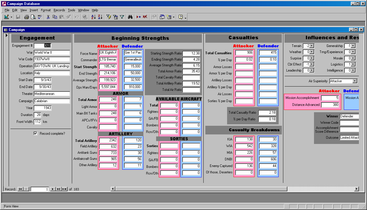
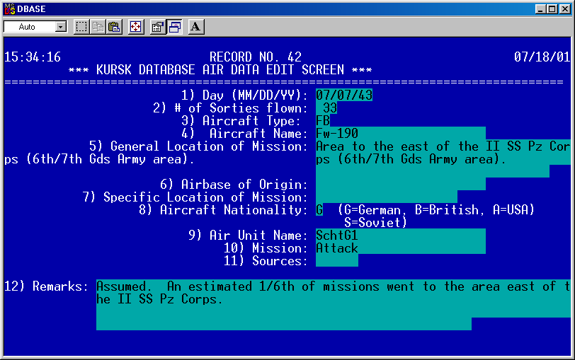
Both the ACSDB and KDB had a significant air component. The air battle over the just the German offensive around Belgorod to the south of Kursk was larger than the Battle of Britain. The Ardennes data base had 1,705 air files. The Kursk data base had 753. One record, from the old Dbase IV version of the Kursk data base, is the picture that starts this blog post. These files basically track every mission for every day, to whatever level of detail the unit records allowed (which were lacking). The air campaign part of these data bases have never been used for any analytical purpose except our preliminary work on creating the Dupuy Air Campaign Model (DACM).
Thanks to a comment made on one of our posts, I recently became aware of a 17 page discussion thread on combat results tables (CRT) that is worth reading. It is here:
By default, much of their discussion of data centers around analysis based upon Trevor Dupuy’s writing, the CBD90 database, the Ardennes Campaign Simulation Data Base (ACSDB), the Kursk Data Base (KDB) and my book War by Numbers. I was not aware of this discussion until yesterday even though the thread was started in 2015 and continues to this year (War by Numbers was published in 2017 so does not appear until the end of page 5 of the thread).
The CBD90 was developed from a Dupuy research effort in the 1980s eventually codified as the Land Warfare Data Base (LWDB). Dupuy’s research was programmed with errors by the government to create the CBD90. A lot of the analysis in my book was based upon a greatly expanded and corrected version of the LWDB. I was the program manager for both the ACSDB and the KDB, and of course, the updated versions of our DuWar suite of combat databases.
There are about a hundred comments I could make to this thread, some in agreement and some in disagreement, but then I would not get my next book finished, so I will refrain. This does not stop me from posting a link:
Allied force dispositions at the Battle of Anzio, on 1 February 1944. [U.S. Army/Wikipedia]
[The article below is reprinted from History, Numbers And War: A HERO Journal, Vol. 1, No. 1, Spring 1977, pp. 34-52]
The Lanchester Equations and Historical Warfare: An Analysis of Sixty World War II Land Engagements
By Janice B. Fain
Background and Objectives
The method by which combat losses are computed is one of the most critical parts of any combat model. The Lanchester equations, which state that a unit’s combat losses depend on the size of its opponent, are widely used for this purpose.
In addition to their use in complex dynamic simulations of warfare, the Lanchester equations have also sewed as simple mathematical models. In fact, during the last decade or so there has been an explosion of theoretical developments based on them. By now their variations and modifications are numerous, and “Lanchester theory” has become almost a separate branch of applied mathematics. However, compared with the effort devoted to theoretical developments, there has been relatively little empirical testing of the basic thesis that combat losses are related to force sizes.
One of the first empirical studies of the Lanchester equations was Engel’s classic work on the Iwo Jima campaign in which he found a reasonable fit between computed and actual U.S. casualties (Note 1). Later studies were somewhat less supportive (Notes 2 and 3), but an investigation of Korean war battles showed that, when the simulated combat units were constrained to follow the tactics of their historical counterparts, casualties during combat could be predicted to within 1 to 13 percent (Note 4).
Taken together, these various studies suggest that, while the Lanchester equations may be poor descriptors of large battles extending over periods during which the forces were not constantly in combat, they may be adequate for predicting losses while the forces are actually engaged in fighting. The purpose of the work reported here is to investigate 60 carefully selected World War II engagements. Since the durations of these battles were short (typically two to three days), it was expected that the Lanchester equations would show a closer fit than was found in studies of larger battles. In particular, one of the objectives was to repeat, in part, Willard’s work on battles of the historical past (Note 3).
The Data Base
Probably the most nearly complete and accurate collection of combat data is the data on World War II compiled by the Historical Evaluation and Research Organization (HERO). From their data HERO analysts selected, for quantitative analysis, the following 60 engagements from four major Italian campaigns:
Salerno, 9-18 Sep 1943, 9 engagements
Volturno, 12 Oct-8 Dec 1943, 20 engagements
Anzio, 22 Jan-29 Feb 1944, 11 engagements
Rome, 14 May-4 June 1944, 20 engagements
The complete data base is described in a HERO report (Note 5). The work described here is not the first analysis of these data. Statistical analyses of weapon effectiveness and the testing of a combat model (the Quantified Judgment Method, QJM) have been carried out (Note 6). The work discussed here examines these engagements from the viewpoint of the Lanchester equations to consider the question: “Are casualties during combat related to the numbers of men in the opposing forces?”
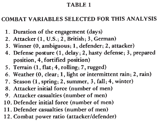
The variables chosen for this analysis are shown in Table 1. The “winners” of the engagements were specified by HERO on the basis of casualties suffered, distance advanced, and subjective estimates of the percentage of the commander’s objective achieved. Variable 12, the Combat Power Ratio, is based on the Operational Lethality Indices (OLI) of the units (Note 7).
The general characteristics of the engagements are briefly described. Of the 60, there were 19 attacks by British forces, 28 by U.S. forces, and 13 by German forces. The attacker was successful in 34 cases; the defender, in 23; and the outcomes of 3 were ambiguous. With respect to terrain, 19 engagements occurred in flat terrain; 24 in rolling, or intermediate, terrain; and 17 in rugged, or difficult, terrain. Clear weather prevailed in 40 cases; 13 engagements were fought in light or intermittent rain; and 7 in medium or heavy rain. There were 28 spring and summer engagements and 32 fall and winter engagements.
Comparison of World War II Engagements With Historical Battles
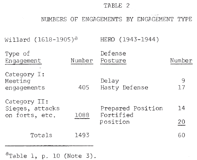
Since one purpose of this work is to repeat, in part, Willard’s analysis, comparison of these World War II engagements with the historical battles (1618-1905) studied by him will be useful. Table 2 shows a comparison of the distribution of battles by type. Willard’s cases were divided into two categories: I. meeting engagements, and II. sieges, attacks on forts, and similar operations. HERO’s World War II engagements were divided into four types based on the posture of the defender: 1. delay, 2. hasty defense, 3. prepared position, and 4. fortified position. If postures 1 and 2 are considered very roughly equivalent to Willard’s category I, then in both data sets the division into the two gross categories is approximately even.
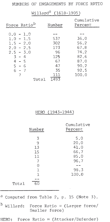
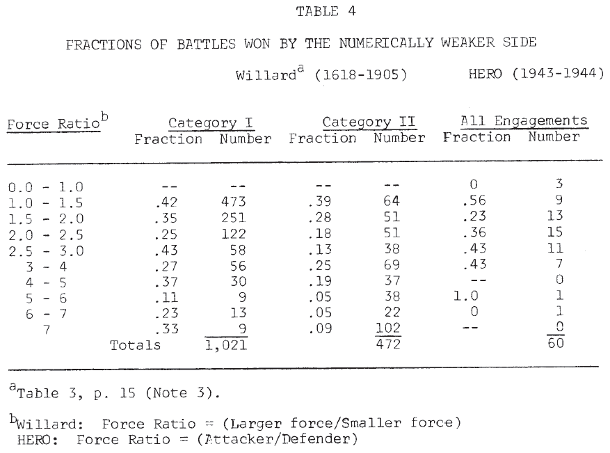
The distribution of engagements across force ratios, given in Table 3, indicated some differences. Willard’s engagements tend to cluster at the lower end of the scale (1-2) and at the higher end (4 and above), while the majority of the World War II engagements were found in mid-range (1.5 – 4) (Note 8). The frequency with which the numerically inferior force achieved victory is shown in Table 4. It is seen that in neither data set are force ratios good predictors of success in battle (Note 9).
Table 3.
Results of the Analysis Willard’s Correlation Analysis
There are two forms of the Lanchester equations. One represents the case in which firing units on both sides know the locations of their opponents and can shift their fire to a new target when a “kill” is achieved. This leads to the “square” law where the loss rate is proportional to the opponent’s size. The second form represents that situation in which only the general location of the opponent is known. This leads to the “linear” law in which the loss rate is proportional to the product of both force sizes.
As Willard points out, large battles are made up of many smaller fights. Some of these obey one law while others obey the other, so that the overall result should be a combination of the two. Starting with a general formulation of Lanchester’s equations, where g is the exponent of the target unit’s size (that is, g is 0 for the square law and 1 for the linear law), he derives the following linear equation:
log (nc/mc) = log E + g log (mo/no) (1)
where nc and mc are the casualties, E is related to the exchange ratio, and mo and no are the initial force sizes. Linear regression produces a value for g. However, instead of lying between 0 and 1, as expected, the) g‘s range from -.27 to -.87, with the majority lying around -.5. (Willard obtains several values for g by dividing his data base in various ways—by force ratio, by casualty ratio, by historical period, and so forth.) A negative g value is unpleasant. As Willard notes:
Military theorists should be disconcerted to find g < 0, for in this range the results seem to imply that if the Lanchester formulation is valid, the casualty-producing power of troops increases as they suffer casualties (Note 3).
From his results, Willard concludes that his analysis does not justify the use of Lanchester equations in large-scale situations (Note 10).
Analysis of the World War II Engagements
Willard’s computations were repeated for the HERO data set. For these engagements, regression produced a value of -.594 for g (Note 11), in striking agreement with Willard’s results. Following his reasoning would lead to the conclusion that either the Lanchester equations do not represent these engagements, or that the casualty producing power of forces increases as their size decreases.
However, since the Lanchester equations are so convenient analytically and their use is so widespread, it appeared worthwhile to reconsider this conclusion. In deriving equation (1), Willard used binomial expansions in which he retained only the leading terms. It seemed possible that the poor results might he due, in part, to this approximation. If the first two terms of these expansions are retained, the following equation results:
log (nc/mc) = log E + log (Mo-mc)/(no-nc) (2)
Repeating this regression on the basis of this equation leads to g = -.413 (Note 12), hardly an improvement over the initial results.
A second attempt was made to salvage this approach. Starting with raw OLI scores (Note 7), HERO analysts have computed “combat potentials” for both sides in these engagements, taking into account the operational factors of posture, vulnerability, and mobility; environmental factors like weather, season, and terrain; and (when the record warrants) psychological factors like troop training, morale, and the quality of leadership. Replacing the factor (mo/no) in Equation (1) by the combat power ratio produces the result) g = .466 (Note 13).
While this is an apparent improvement in the value of g, it is achieved at the expense of somewhat distorting the Lanchester concept. It does preserve the functional form of the equations, but it requires a somewhat strange definition of “killing rates.”
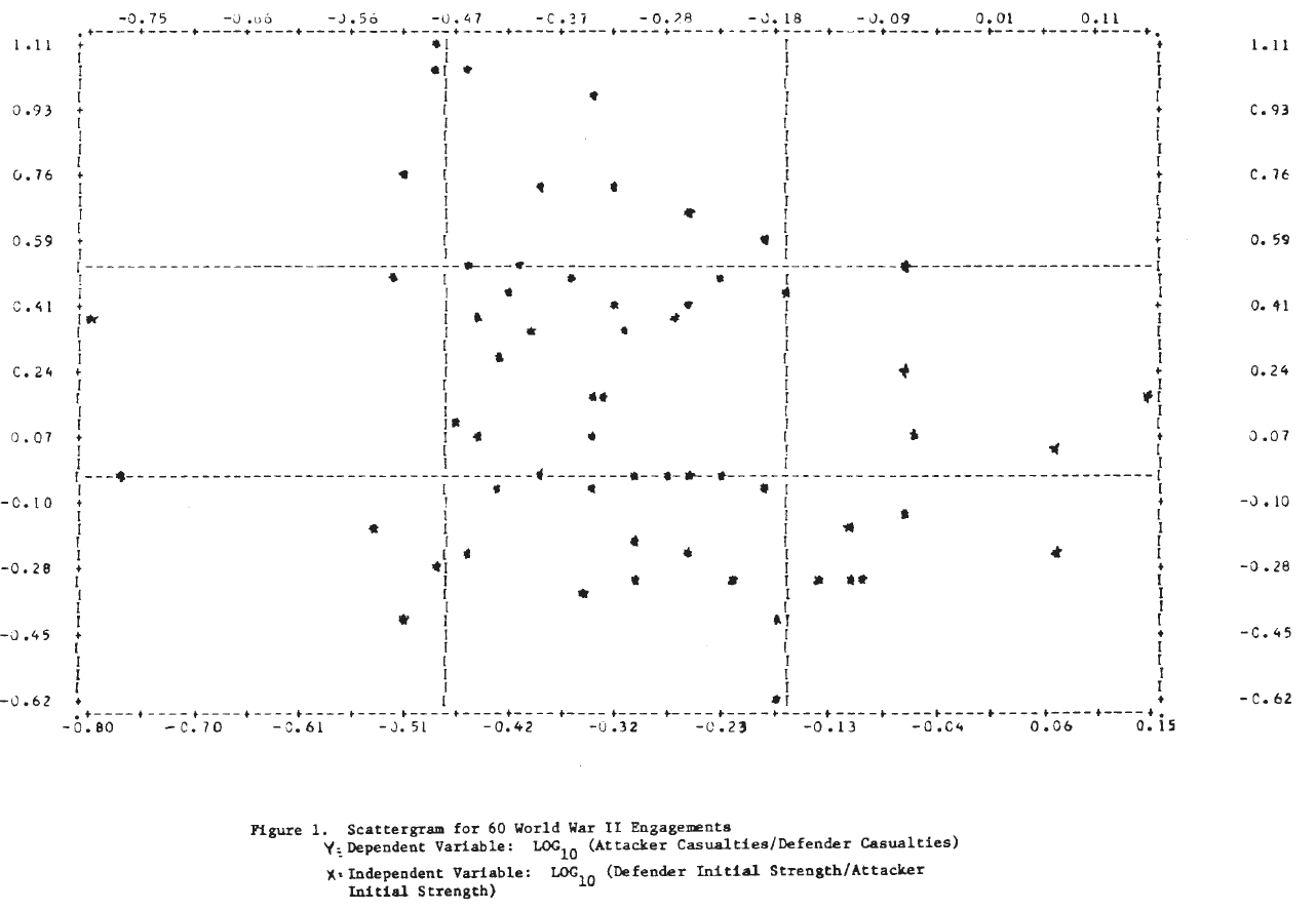
Analysis Based on the Differential Lanchester Equations
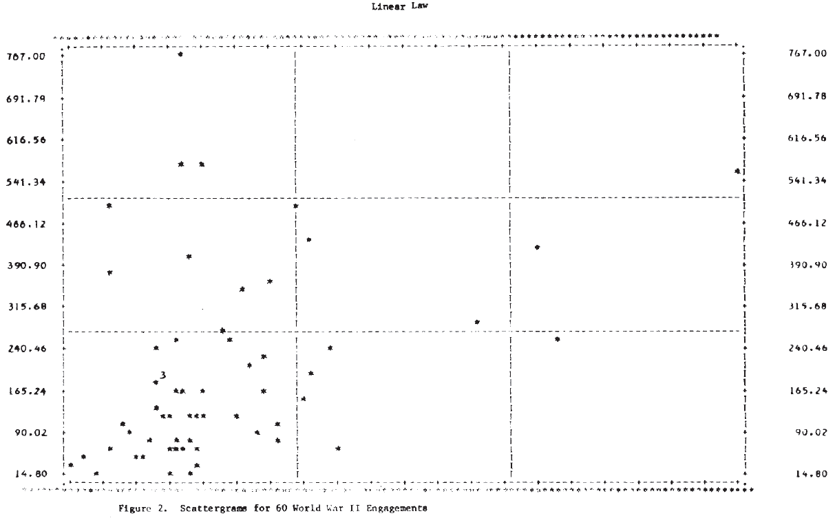
Analysis of the type carried out by Willard appears to produce very poor results for these World War II engagements. Part of the reason for this is apparent from Figure 1, which shows the scatterplot of the dependent variable, log (nc/mc), against the independent variable, log (mo/no). It is clear that no straight line will fit these data very well, and one with a positive slope would not be much worse than the “best” line found by regression. To expect the exponent to account for the wide variation in these data seems unreasonable.
Here, a simpler approach will be taken. Rather than use the data to attempt to discriminate directly between the square and the linear laws, they will be used to estimate linear coefficients under each assumption in turn, starting with the differential formulation rather than the integrated equations used by Willard.
In their simplest differential form, the Lanchester equations may be written;
Square Law; dA/dt = -kdD and dD/dt = kaA (3)
Linear law: dA/dt = -k’dAD and dD/dt = k’aAD (4)
where
A(D) is the size of the attacker (defender)
dA/dt (dD/dt) is the attacker’s (defender’s) loss rate,
ka, k’a (kd, k’d) are the attacker’s (defender’s) killing rates
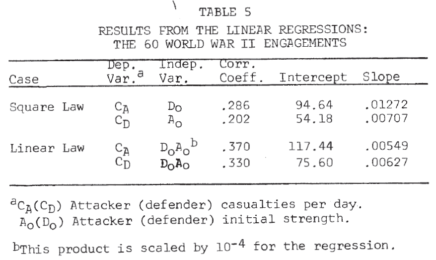
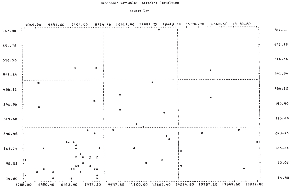
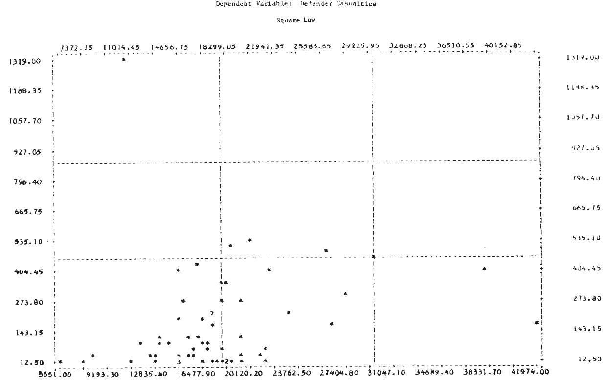
For this analysis, the day is taken as the basic time unit, and the loss rate per day is approximated by the casualties per day. Results of the linear regressions are given in Table 5. No conclusions should be drawn from the fact that the correlation coefficients are higher in the linear law case since this is expected for purely technical reasons (Note 14). A better picture of the relationships is again provided by the scatterplots in Figure 2. It is clear from these plots that, as in the case of the logarithmic forms, a single straight line will not fit the entire set of 60 engagements for either of the dependent variables.
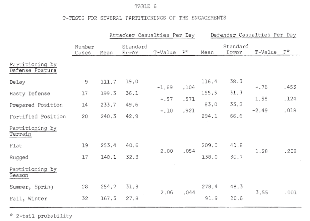
To investigate ways in which the data set might profitably be subdivided for analysis, T-tests of the means of the dependent variable were made for several partitionings of the data set. The results, shown in Table 6, suggest that dividing the engagements by defense posture might prove worthwhile.
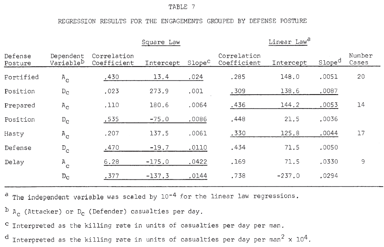
Results of the linear regressions by defense posture are shown in Table 7. For each posture, the equation that seemed to give a better fit to the data is underlined (Note 15). From this table, the following very tentative conclusions might be drawn:
In an attack on a fortified position, the attacker suffers casualties by the square law; the defender suffers casualties by the linear law. That is, the defender is aware of the attacker’s position, while the attacker knows only the general location of the defender. (This is similar to Deitchman’s guerrilla model. Note 16).
This situation is apparently reversed in the cases of attacks on prepared positions and hasty defenses.
Delaying situations seem to be treated better by the square law for both attacker and defender.
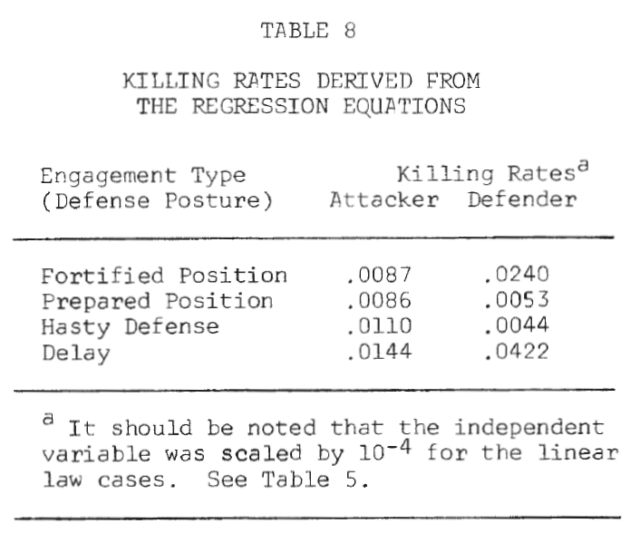
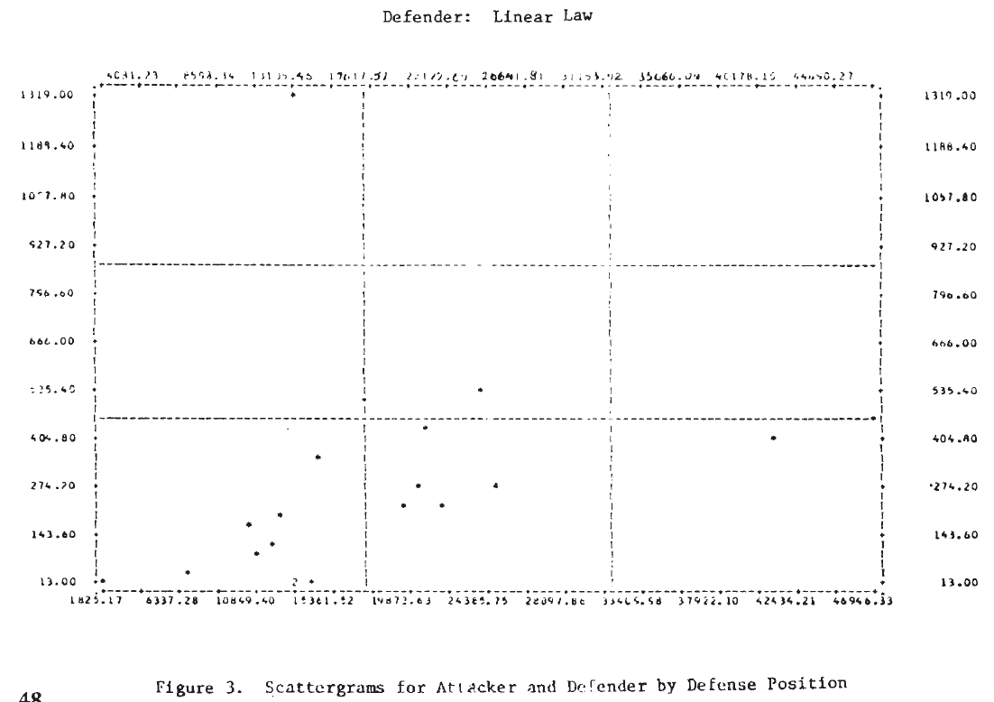
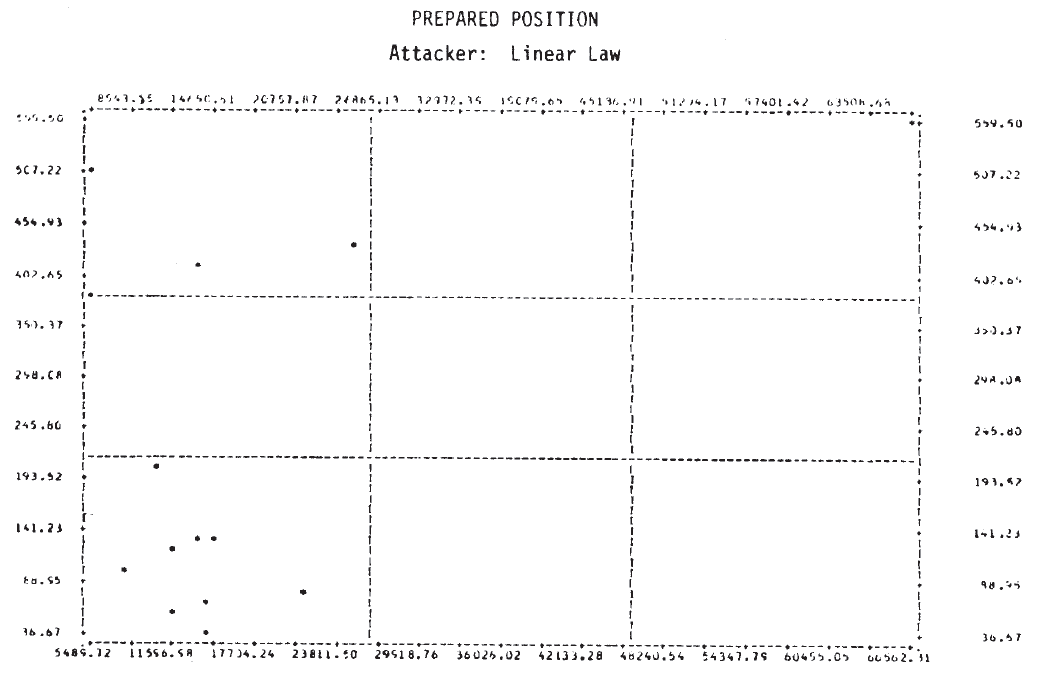
Table 8 summarizes the killing rates by defense posture. The defender has a much higher killing rate than the attacker (almost 3 to 1) in a fortified position. In a prepared position and hasty defense, the attacker appears to have the advantage. However, in a delaying action, the defender’s killing rate is again greater than the attacker’s (Note 17).
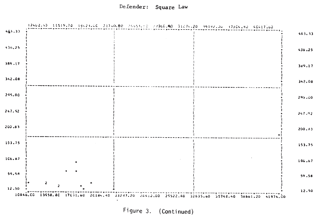
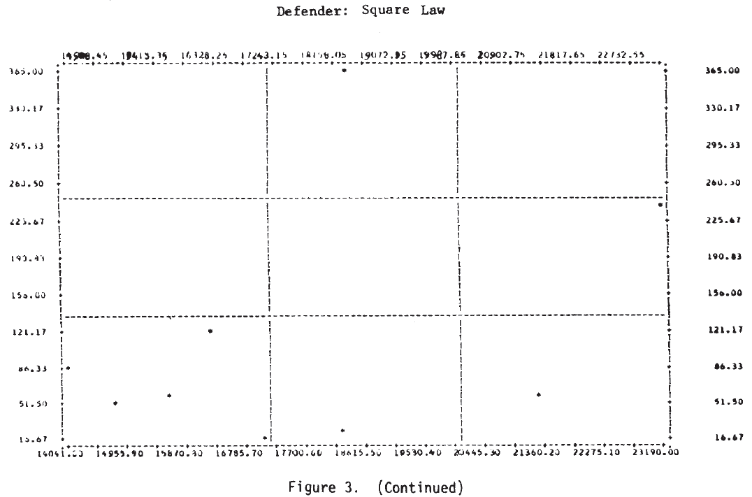
Figure 3 shows the scatterplots for these cases. Examination of these plots suggests that a tentative answer to the study question posed above might be: “Yes, casualties do appear to be related to the force sizes, but the relationship may not be a simple linear one.”
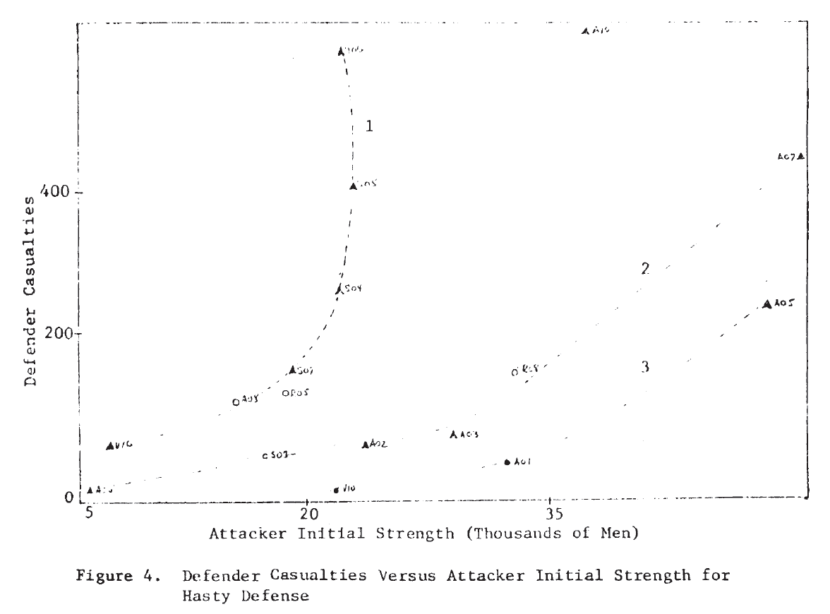
In several of these plots it appears that two or more functional forms may be involved. Consider, for example, the defender‘s casualties as a function of the attacker’s initial strength in the case of a hasty defense. This plot is repeated in Figure 4, where the points appear to fit the curves sketched there. It would appear that there are at least two, possibly three, separate relationships. Also on that plot, the individual engagements have been identified, and it is interesting to note that on the curve marked (1), five of the seven attacks were made by Germans—four of them from the Salerno campaign. It would appear from this that German attacks are associated with higher than average defender casualties for the attacking force size. Since there are so few data points, this cannot be more than a hint or interesting suggestion.
Future Research
This work suggests two conclusions that might have an impact on future lines of research on combat dynamics:
Tactics appear to be an important determinant of combat results. This conclusion, in itself, does not appear startling, at least not to the military. However, it does not always seem to have been the case that tactical questions have been considered seriously by analysts in their studies of the effects of varying force levels and force mixes.
Historical data of this type offer rich opportunities for studying the effects of tactics. For example, consideration of the narrative accounts of these battles might permit re-coding the engagements into a larger, more sensitive set of engagement categories. (It would, of course, then be highly desirable to add more engagements to the data set.)
While predictions of the future are always dangerous, I would nevertheless like to suggest what appears to be a possible trend. While military analysis of the past two decades has focused almost exclusively on the hardware of weapons systems, at least part of our future analysis will be devoted to the more behavioral aspects of combat.
Janice Bloom Fain, a Senior Associate of CACI, lnc., is a physicist whose special interests are in the applications of computer simulation techniques to industrial and military operations; she is the author of numerous reports and articles in this field. This paper was presented by Dr. Fain at the Military Operations Research Symposium at Fort Eustis, Virginia.
[5.] HERO, “A Study of the Relationship of Tactical Air Support Operations to Land Combat, Appendix B, Historical Data Base.” Historical Evaluation and Research Organization, report prepared for the Defense Operational Analysis Establishment, U.K.T.S.D., Contract D-4052 (1971).
[6.] T. N. Dupuy, The Quantified Judgment Method of Analysis of Historical Combat Data, HERO Monograph, (January 1973); HERO, “Statistical Inference in Analysis in Combat,” Annex F, Historical Data Research on Tactical Air Operations, prepared for Headquarters USAF, Assistant Chief of Staff for Studies and Analysis, Contract No. F-44620-70-C-0058 (1972).
[7.] The Operational Lethality Index (OLI) is a measure of weapon effectiveness developed by HERO.
[8.] Since Willard’s data did not indicate which side was the attacker, his force ratio is defined to be (larger force/smaller force). The HERO force ratio is (attacker/defender).
[9.] Since the criteria for success may have been rather different for the two sets of battles, this comparison may not be very meaningful.
[10.] This work includes more complex analysis in which the possibility that the two forces may be engaging in different types of combat is considered, leading to the use of two exponents rather than the single one, Stochastic combat processes are also treated.
[11.] Correlation coefficient = -.262;
Intercept = .00115; slope = -.594.
[12.] Correlation coefficient = -.184;
Intercept = .0539; slope = -,413.
[13.] Correlation coefficient = .303;
Intercept = -.638; slope = .466.
[14.] Correlation coefficients for the linear law are inflated with respect to the square law since the independent variable is a product of force sizes and, thus, has a higher variance than the single force size unit in the square law case.
[15.] This is a subjective judgment based on the following considerations Since the correlation coefficient is inflated for the linear law, when it is lower the square law case is chosen. When the linear law correlation coefficient is higher, the case with the intercept closer to 0 is chosen.
[17.] As pointed out by Mr. Alan Washburn, who prepared a critique on this paper, when comparing numerical values of the square law and linear law killing rates, the differences in units must be considered. (See footnotes to Table 7).
Over the years I have run across a number of Australian Operations Research and Historical Analysis efforts. Overall, I have been impressed with what I have seen. Below is one of their papers written by Nigel Perry. He is not otherwise known to me. It is dated December 2011: Applications of Historical Analyses in Combat Modeling
It does address the value of Lanchester equations in force-on-force combat models, which in my mind is already a settled argument (see: Lanchester Equations Have Been Weighed). His is the latest argument that I gather reinforces this point.
The author of this paper references the work of Robert Helmbold and Dean Hartley (see page 14). He does favorably reference the work of Trevor Dupuy but does not seem to be completely aware of the extent or full nature of it (pages 14, 16, 17, 24 and 53). He does not seem to aware that the work of Helmbold and Hartley was both built from a database that was created by Trevor Dupuy’s companies HERO & DMSI. Without Dupuy, Helmbold and Hartley would not have had data to work from.
Specifically, Helmbold was using the Chase database, which was programmed by the government from the original paper version provided by Dupuy. I think it consisted of 597-599 battles (working from memory here). It also included a number of coding errors when they programmed it and did not include the battle narratives. Hartley had Oakridge National Laboratories purchase a computerized copy from Dupuy of what was now called the Land Warfare Data Base (LWDB). It consisted of 603 or 605 engagements (and did not have the coding errors but still did not include the narratives). As such, they both worked from almost the same databases.
Dr. Perrty does take a copy of Hartley’s database and expands it to create more engagements. He says he expanded it from 750 battles (except the database we sold to Harley had 603 or 605 cases) to around 1600. It was estimated in the 1980s by Curt Johnson (Director and VP of HERO) to take three man-days to create a battle. If this estimate is valid (actually I think it is low), then to get to 1600 engagements the Australian researchers either invested something like 10 man-years of research, or relied heavily on secondary sources without any systematic research, or only partly developed each engagement (for example, only who won and lost). I suspect the latter.
Post WWII………….1950……..2008…………118……………….86…………….32
We, of course, did something very similar. We took the Land Warfare Data Base (the 605 engagement version), expanded in considerably with WWII and post-WWII data, proofed and revised a number of engagements using more primarily source data, divided it into levels of combat (army-level, division-level, battalion-level, company-level) and conducted analysis with the 1280 or so engagements we had. This was a much more powerful and better organized tool. We also looked at winner and loser, but used the 605 engagement version (as we did the analysis in 1996). An example of this, from pages 16 and 17 of my manuscript for War by Numbers shows:
Attacker Won:
Force Ratio Force Ratio Percent Attack Wins:
Greater than or less than Force Ratio Greater Than
equal to 1-to-1 1-to1 or equal to 1-to-1
1600-1699 16 18 47%
1700-1799 25 16 61%
1800-1899 47 17 73%
1900-1920 69 13 84%
1937-1945 104 8 93%
1967-1973 17 17 50%
Total 278 89 76%
Defender Won:
Force Ratio Force Ratio Percent Defense Wins:
Greater than or less than Force Ratio Greater Than
equal to 1-to-1 1-to1 or equal to 1-to-1
1600-1699 7 6 54%
1700-1799 11 13 46%
1800-1899 38 20 66%
1900-1920 30 13 70%
1937-1945 33 10 77%
1967-1973 11 5 69%
Total 130 67 66%
Anyhow, from there (pages 26-59) the report heads into an extended discussion of the analysis done by Helmbold and Hartley (which I am not that enamored with). My book heads in a different direction: War by Numbers III (Table of Contents)
He actually tested his equations to historical data, which are presented in his paper. He ended up coming up with something similar to Lanchester equations but it did not have a square law, but got a similar effect by putting things to the 3/2nds power.
As far as we know, because of the time it was published (June-October 1915), it was not influenced or done with any awareness of work that the far more famous Frederick Lanchester had done (and Lanchester was famous for a lot more than just his modeling equations). Lanchester first published his work in the fall of 1914 (after the Great War had already started). It is possible that Osipov was aware of it, but he does not mention Lanchester. He was probably not aware of Lanchester’s work. It appears to be the case of him independently coming up with the use of differential equations to describe combat attrition. This was also the case with Rear Admiral J. V. Chase, who wrote a classified staff paper for U.S. Navy in 1902 that was not revealed until 1972.
Osipov, after he had written his paper, may have served in World War I, which was already underway at the time it was published. Between the war, the Russian revolutions, the civil war afterwards, the subsequent repressions by Cheka and later Stalin, we do not know what happened to M. Osipov. At the time I was asked by CAA if our Russian research team knew about him. I passed the question to Col. Sverdlov and Col. Vainer and they were not aware of him. It is probably possible to chase him down, but would probably take some effort. Perhaps some industrious researcher will find out more about him.
It does not appear that Osipov had any influence on Soviet operations research or military analysis. It appears that he was ignored or forgotten. His article was re-published in the September 1988 of the Soviet Military-Historical Journal with the propaganda influenced statement that they also had their own “Lanchester.” Of course, this “Soviet Lanchester” was publishing in a Tsarist military journal, hardly a demonstration of the strength of the Soviet system.