People do send me some damn interesting stuff. Someone just sent me a page clipped from U.S. Army FM 3-0 Operations, dated 6 October 2017. There is a discussion in Chapter 7 on “penetration.” This brief discussion on paragraph 7-115 states in part:
7-115. A penetration is a form of maneuver in which an attacking force seeks to rupture enemy defenses on a narrow front to disrupt the defensive system (FM 3-90-1) ….The First U.S. Army’s Operation Cobra (the breakout from the Normandy lodgment in July 1944) is a classic example of a penetration. Figure 7-10 illustrates potential correlation of forces or combat power for a penetration…..”
This is figure 7-10:
So:
Corps shaping operations: 3:1
Corps decisive operations: 9-1
Lead battalion: 18-1
Now, in contrast, let me pull some material from War by Numbers:
From page 10:
European Theater of Operations (ETO) Data, 1944
Force Ratio Result Percent Failure Number of cases
0.55 to 1.01-to-1.00 Attack Fails 100% 5
1.15 to 1.88-to-1.00 Attack usually succeeds 21% 48
1.95 to 2.56-to-1.00 Attack usually succeeds 10% 21
2.71-to-1.00 and higher Attacker Advances 0% 42
Note that these are division-level engagements. I guess I could assemble the same data for corps-level engagements, but I don’t think it would look much different.
From page 210:
Force Ratio…………Cases……Terrain…….Result
1.18 to 1.29 to 1 4 Nonurban Defender penetrated
1.51 to 1.64 3 Nonurban Defender penetrated
2.01 to 2.64 2 Nonurban Defender penetrated
3.03 to 4.28 2 Nonurban Defender penetrated
4.16 to 4.78 2 Urban Defender penetrated
6.98 to 8.20 2 Nonurban Defender penetrated
6.46 to 11.96 to 1 2 Urban Defender penetrated
These are also division-level engagements from the ETO. One will note that out of 17 cases where the defender was penetrated, only once was the force ratio as high as 9 to 1. The mean force ratio for these 17 cases is 3.77 and the median force ratio is 2.64.
Now the other relevant tables in this book are in Chapter 8: Outcome of Battles (page 60-71). There I have a set of tables looking at the loss rates based upon one of six outcomes. Outcome V is defender penetrated. Unfortunately, as the purpose of the project was to determine prisoner of war capture rates, we did not bother to calculate the average force ratio for each outcome. But, knowing the database well, the average force ratio for defender penetrated results may be less than 3-to-1 and is certainly is less than 9-to-1. Maybe I will take few days at some point and put together a force ratio by outcome table.
Now, the source of FM 3.0 data is not known to us and is not referenced in the manual. Why they don’t provide such a reference is a mystery to me, as I can point out several examples of this being an issue. On more than one occasion data has appeared in Army manuals that we can neither confirm or check, and which we could never find the source for. But…it is not referenced. I have not looked at the operation in depth, but don’t doubt that at some point during Cobra they had a 9:1 force ratio and achieved a penetration. But…..this is different than leaving the impression that a 9:1 force ratio is needed to achieve a penetration. I do not know it that was the author’s intent, but it is something that the casual reader might infer. This probably needs to be clarified.
Reilly starts with a very nice statement of the issue:
Clearly breakpoints are crucial when modelling battlefield combat. I have read extensively about it using mostly first hand accounts of battles rather than high level summaries. Some of the major factors causing it appear to be loss of leadership (e.g. Harald’s death at Hastings), loss of belief in the units capacity to achieve its objectives (e.g. the retreat of the Old Guard at Waterloo, surprise often figured in Mongol successes, over confidence resulting in impetuous attacks which fail dramatically (e.g. French attacks at Agincourt and Crecy), loss of control over the troops (again Crecy and Agincourt) are some of the main ones I can think of off hand.
The break-point crisis seems to occur against a background of confusion, disorder, mounting casualties, increasing fatigue and loss of morale. Casualties are part of the background but not usually the actual break point itself.
He then states:
Perhaps a way forward in the short term is to review a number of first hand battle accounts (I am sure you can think of many) and calculate the percentage of times these factors and others appear as breakpoints in the literature.
This has been done. In effect this is what Robert McQuie did in his article and what was the basis for the DMSI breakpoints study.
Why wait for the military to do something? You will die of old age before that happens!
That is distinctly possible. If this really was a simple issue that one person working for a year could produce a nice definitive answer for…..it would have already been done !!!
Let us look at the 1988 Breakpoints study. There was some effort leading up to that point. Trevor Dupuy and DMSI had already looked into the issue. This included developing a database of engagements (the Land Warfare Data Base or LWDB) and using that to examine the nature of breakpoints. The McQuie article was developed from this database, and his article was closely coordinated with Trevor Dupuy. This was part of the effort that led to the U.S. Army’s Concepts Analysis Agency (CAA) to issue out a RFP (Request for Proposal). It was competitive. I wrote the proposal that won the contract award, but the contract was given to Dr. Janice Fain to lead. My proposal was more quantitative in approach than what she actually did. Her effort was more of an intellectual exploration of the issue. I gather this was done with the assumption that there would be a follow-on contract (there never was). Now, up until that point at least a man-year of effort had been expended, and if you count the time to develop the databases used, it was several man-years.
Now the Breakpoints study was headed up by Dr. Janice B. Fain, who worked on it for the better part of a year. Trevor N. Dupuy worked on it part-time. Gay M. Hammerman conducted the interview with the veterans. Richard C. Anderson researched and created an additional 24 engagements that had clear breakpoints in them for the study (that is DMSI report 117B). Charles F. Hawkins was involved in analyzing the engagements from the LWDB. There were several other people also involved to some extent. Also, 39 veterans were interviewed for this effort. Many were brought into the office to talk about their experiences (that was truly entertaining). There were also a half-dozen other staff members and consultants involved in the effort, including Lt. Col. James T. Price (USA, ret), Dr. David Segal (sociologist), Dr. Abraham Wolf (a research psychologist), Dr. Peter Shapiro (social psychology) and Col. John R. Brinkerhoff (USA, ret). There were consultant fees, travel costs and other expenses related to that. So, the entire effort took at least three “man-years” of effort. This was what was needed just get to the point where we are able to take the next step.
This is not something that a single scholar can do. That is why funding is needed.
As to dying of old age before that happens…..that may very well be the case. Right now, I am working on two books, one of them under contract. I sort of need to finish those up before I look at breakpoints again. After that, I will decide whether to work on a follow-on to America’s Modern Wars (called Future American Wars) or work on a follow-on to War by Numbers (called War by Numbers II…being the creative guy that I am). Of course, neither of these books are selling well….so perhaps my time would be better spent writing another Kursk book, or any number of other interesting projects on my plate. Anyhow, if I do War by Numbers II, then I do plan on investing several chapters into addressing breakpoints. This would include using the 1,000+ cases that now populate our combat databases to do some analysis. This is going to take some time. So…….I may get to it next year or the year after that, but I may not. If someone really needs the issue addressed, they really need to contract for it.
A breakpoint or involuntary change in posture is an essential part of modeling. There is a breakpoint methodology in C-WAM. According to slide 18 and rule book section 5.7.2 is that ground unit below 50% strength can only defend. It is removed at below 30% strength. I gather this is a breakpoint for a brigade.
Let me just quote from Chapter 18 (Modeling Warfare) of my book War by Numbers: Understanding Conventional Combat (pages 288-289):
The original breakpoints study was done in 1954 by Dorothy Clark of ORO [which can be found here].[1] It examined forty-three battalion-level engagements where the units “broke,” including measuring the percentage of losses at the time of the break. Clark correctly determined that casualties were probably not the primary cause of the breakpoint and also declared the need to look at more data. Obviously, forty-three cases of highly variable social science-type data with a large number of variables influencing them are not enough for any form of definitive study. Furthermore, she divided the breakpoints into three categories, resulting in one category based upon only nine observations. Also, as should have been obvious, this data would apply only to battalion-level combat. Clark concluded “The statement that a unit can be considered no longer combat effective when it has suffered a specific casualty percentage is a gross oversimplification not supported by combat data.” She also stated “Because of wide variations in data, average loss percentages alone have limited meaning.”[2]
Yet, even with her clear rejection of a percent loss formulation for breakpoints, the 20 to 40 percent casualty breakpoint figures remained in use by the training and combat modeling community. Charts in the 1964 Maneuver Control field manual showed a curve with the probability of unit break based on percentage of combat casualties.[3] Once a defending unit reached around 40 percent casualties, the chance of breaking approached 100 percent. Once an attacking unit reached around 20 percent casualties, the chance of it halting (type I break) approached 100% and the chance of it breaking (type II break) reached 40 percent. These data were for battalion-level combat. Because they were also applied to combat models, many models established a breakpoint of around 30 or 40 percent casualties for units of any size (and often applied to division-sized units).
To date, we have absolutely no idea where these rule-of-thumb formulations came from and despair of ever discovering their source. These formulations persist despite the fact that in fifteen (35%) of the cases in Clark’s study, the battalions had suffered more than 40 percent casualties before they broke. Furthermore, at the division-level in World War II, only two U.S. Army divisions (and there were ninety-one committed to combat) ever suffered more than 30% casualties in a week![4] Yet, there were many forced changes in combat posture by these divisions well below that casualty threshold.
The next breakpoints study occurred in 1988.[5] There was absolutely nothing of any significance (meaning providing any form of quantitative measurement) in the intervening thirty-five years, yet there were dozens of models in use that offered a breakpoint methodology. The 1988 study was inconclusive, and since then nothing further has been done.[6]
This seemingly extreme case is a fairly typical example. A specific combat phenomenon was studied only twice in the last fifty years, both times with inconclusive results, yet this phenomenon is incorporated in most combat models. Sadly, similar examples can be pulled for virtually each and every phenomena of combat being modeled. This failure to adequately examine basic combat phenomena is a problem independent of actual combat modeling methodology.
[3] Headquarters, Department of the Army, FM 105-5 Maneuver Control (Washington, D.C., December, 1967), pages 128-133.
[4] The two exceptions included the U.S. 106th Infantry Division in December 1944, which incidentally continued fighting in the days after suffering more than 40 percent losses, and the Philippine Division upon its surrender in Bataan on 9 April 1942 suffered 100% losses in one day in addition to very heavy losses in the days leading up to its surrender.
[5] This was HERO Report number 117, Forced Changes of Combat Posture (Breakpoints) (Historical Evaluation and Research Organization, Fairfax, VA., 1988). The intervening years between 1954 and 1988 were not entirely quiet. See HERO Report number 112, Defeat Criteria Seminar, Seminar Papers on the Evaluation of the Criteria for Defeat in Battle (Historical Evaluation and Research Organization, Fairfax, VA., 12 June 1987) and the significant article by Robert McQuie, “Battle Outcomes: Casualty Rates as a Measure of Defeat” in Army, issue 37 (November 1987). Some of the results of the 1988 study was summarized in the book by Trevor N. Dupuy, Understanding Defeat: How to Recover from Loss in Battle to Gain Victory in War (Paragon House Publishers, New York, 1990).
[6] The 1988 study was the basis for Trevor Dupuy’s book: Col. T. N. Dupuy, Understanding Defeat: How to Recover From Loss in Battle to Gain Victory in War (Paragon House Publishers, New York, 1990).
In an exchange with one of readers, he mentioned that about the possibility to quantifiably access the performances of armies and produce a ranking from best to worst. The exchange is here:
We have done some work on this, and are the people who have done the most extensive published work on this. Swedish researcher Niklas Zetterling in his book Normandy 1944: German Military Organization, Combat Power and Organizational Effectiveness also addresses this subject, as he has elsewhere, for example, an article in The International TNDM Newsletter, volume I, No. 6, pages 21-23 called “CEV Calculations in Italy, 1943.” It is here: http://www.dupuyinstitute.org/tdipub4.htm
When it came to measuring the differences in performance of armies, Martin van Creveld referenced Trevor Dupuy in his book Fighting Power: German and U.S. Army Performance, 1939-1945, pages 4-8.
What Trevor Dupuy has done is compare the performances of both overall forces and individual divisions based upon his Quantified Judgment Model (QJM). This was done in his book Numbers, Predictions and War: The Use of History to Evaluate and Predict the Outcome of Armed Conflict. I bring the readers attention to pages ix, 62-63, Chapter 7: Behavioral Variables in World War II (pages 95-110), Chapter 9: Reliably Representing the Arab-Israeli Wars (pages 118-139), and in particular page 135, and pages 163-165. It was also discussed in Understanding War: History and Theory of Combat, Chapter Ten: Relative Combat Effectiveness (pages 105-123).
I ended up dedicating four chapters in my book War by Numbers: Understanding Conventional Combat to the same issue. One of the problems with Trevor Dupuy’s approach is that you had to accept his combat model as a valid measurement of unit performance. This was a reach for many people, especially those who did not like his conclusions to start with. I choose to simply use the combined statistical comparisons of dozens of division-level engagements, which I think makes the case fairly convincingly without adding a construct to manipulate the data. If someone has a disagreement with my statistical compilations and the results and conclusions from it, I have yet to hear them. I would recommend looking at Chapter 4: Human Factors (pages 16-18), Chapter 5: Measuring Human Factors in Combat: Italy 1943-1944 (pages 19-31), Chapter 6: Measuring Human Factors in Combat: Ardennes and Kursk (pages 32-48), and Chapter 7: Measuring Human Factors in Combat: Modern Wars (pages 49-59).
Now, I did end up discussing Trevor Dupuy’s model in Chapter 19: Validation of the TNDM and showing the results of the historical validations we have done of his model, but the model was not otherwise used in any of the analysis done in the book.
But….what we (Dupuy and I) have done is a comparison between forces that opposed each other. It is a measurement of combat value relative to each other. It is not an absolute measurement that can be compared to other armies in different times and places. Trevor Dupuy toyed with this on page 165 of NPW, but this could only be done by assuming that combat effectiveness of the U.S. Army in WWII was the same as the Israeli Army in 1973.
Anyhow, it is probably impossible to come up with a valid performance measurement that would allow you to rank an army from best to worse. It is possible to come up with a comparative performance measurement of armies that have faced each other. This, I believe we have done, using different methodologies and different historical databases. I do believe it would be possible to then determine what the different factors are that make up this difference. I do believe it would be possible to assign values or weights to those factors. I believe this would be very useful to know, in light of the potential training and organizational value of this knowledge.
We do have World War I engagements in our databases and have included in some of our analysis. We have done some other research related to World War I (funded by the UK Ministry of Defence, of course):
Instead of responding in the comments section, I have decided to respond with another blog post.
As the person points out, most Army simulations exist to “enable students/staff to maintain and improve readiness…improve their staff skills, SOPs, reporting procedures, and planning….”
Yes this true, but I argue that this does not obviate the need for accurate simulations. Assuming no change in complexity, I cannot think of a single scenario where having a less accurate model is more desirable that having a more accurate model.
Now what is missing from many of these models that I have seen? Often a realistic unit breakpoint methodology, a proper comparison of force ratios, a proper set of casualty rates, addressing human factors, and many other matters. Many of these things are being done in these simulations already, but are being done incorrectly. Quite simply, they do not realistically portray a range of historical or real combat examples.
He then quotes the 1997-1998 Simulation Handbook of the National Simulations Training Center:
The algorithms used in training simulations provide sufficient fidelity for training, not validation of war plans. This is due to the fact that important factors (leadership, morale, terrain, weather, level of training or units) and a myriad of human and environmental impacts are not modeled in sufficient detail….”
Let’s take their list made around 20 years ago. In the last 20 years, what significant quantitative studies have been done on the impact of leadership on combat? Can anyone list them? Can anyone point to even one? The same with morale or level of training of units. The Army has TRADOC, the Army Staff, Leavenworth, the War College, CAA and other agencies, and I have not seen in the last twenty years a quantitative study done to address these issues. And what of terrain and weather? They have been around for a long time.
Army simulations have been around since the late 1950s. So at the time these shortfalls are noted in 1997-1998, 40 years had passed. By their own admission, these issues had not been adequately addressed in the previous 40 years. I gather they have not been adequately in addressed in the last 20 years. So, the clock is ticking, 60 years of Army modeling and simulation, and no one has yet fully and properly address many of these issues. In many cases, they have not even gotten a good start in addressing them.
Anyhow, I have little interest in arguing these issues. My interest is in correcting them.
Technology and the Human Factor in War by Trevor N. Dupuy
The Debate
It has become evident to many military theorists that technology has become increasingly important in war. In fact (even though many soldiers would not like to admit it) most such theorists believe that technology has actually reduced the significance of the human factor in war, In other words, the more advanced our military technology, these “technocrats” believe, the less we need to worry about the professional capability and competence of generals, admirals, soldiers, sailors, and airmen.
The technocrats believe that the results of the Kuwait, or Gulf, War of 1991 have confirmed their conviction. They cite the contribution to those results of the U.N. (mainly U.S.) command of the air, stealth aircraft, sophisticated guided missiles, and general electronic superiority, They believe that it was technology which simply made irrelevant the recent combat experience of the Iraqis in their long war with Iran.
Yet there are a few humanist military theorists who believe that the technocrats have totally misread the lessons of this century‘s wars! They agree that, while technology was important in the overwhelming U.N. victory, the principal reason for the tremendous margin of U.N. superiority was the better training, skill, and dedication of U.N. forces (again, mainly U.S.).
And so the debate rests. Both sides believe that the result of the Kuwait War favors their point of view, Nevertheless, an objective assessment of the literature in professional military journals, of doctrinal trends in the U.S. services, and (above all) of trends in the U.S. defense budget, suggest that the technocrats have stronger arguments than the humanists—or at least have been more convincing in presenting their arguments.
I suggest, however, that a completely impartial comparison of the Kuwait War results with those of other recent wars, and with some of the phenomena of World War II, shows that the humanists should not yet concede the debate.
I am a humanist, who is also convinced that technology is as important today in war as it ever was (and it has always been important), and that any national or military leader who neglects military technology does so to his peril and that of his country, But, paradoxically, perhaps to an extent even greater than ever before, the quality of military men is what wins wars and preserves nations.
To elevate the debate beyond generalities, and demonstrate convincingly that the human factor is at least as important as technology in war, I shall review eight instances in this past century when a military force has been successful because of the quality if its people, even though the other side was at least equal or superior in the technological sophistication of its weapons. The examples I shall use are:
Germany vs. the USSR in World War II
Germany vs. the West in World War II
Israel vs. Arabs in 1948, 1956, 1967, 1973 and 1982
The Vietnam War, 1965-1973
Britain vs. Argentina in the Falklands 1982
South Africans vs. Angolans and Cubans, 1987-88
The U.S. vs. Iraq, 1991
The demonstration will be based upon a marshaling of historical facts, then analyzing those facts by means of a little simple arithmetic.
Relative Combat Effectiveness Value (CEV)
The purpose of the arithmetic is to calculate relative combat effectiveness values (CEVs) of two opposing military forces. Let me digress to set up the arithmetic. Although some people who hail from south of the Mason-Dixon Line may be reluctant to accept the fact, statistics prove that the fighting quality of Northern soldiers and Southern soldiers was virtually equal in the American Civil War. (I invite those who might disagree to look at Livermore’s Numbers and Losses in the Civil War). That assumption of equality of the opposing troop quality in the Civil War enables me to assert that the successful side in every important battle in the Civil War was successful either because of numerical superiority or superior generalship. Three of Lee’s battles make the point:
Despite being outnumbered, Lee won at Antietam. (Though Antietam is sometimes claimed as a Union victory, Lee, the defender, held the battlefield; McClellan, the attacker, was repulsed.) The main reason for Lee’s success was that on a scale of leadership his generalship was worth 10, while McClellan was barely a 6.
Despite being outnumbered, Lee won at Chancellorsville because he was a 10 to Hooker’s 5.
Lee lost at Gettysburg mainly because he was outnumbered. Also relevant: Meade did not lose his nerve (like McClellan and Hooker) with generalship worth 8 to match Lee’s 8.
Let me use Antietam to show the arithmetic involved in those simple analyses of a rather complex subject:
The numerical strength of McClellan’s army was 89,000; Lee’s army was only 39,000 strong, but had the multiplier benefit of defensive posture. This enables us to calculate the theoretical combat power ratio of the Union Army to the Confederate Army as 1.4:1.0. In other words, with substantial preponderance of force, the Union Army should have been successful. (The combat power ratio of Confederates to Northerners, of course, was the reciprocal, or 0.71:1.04)
However, Lee held the battlefield, and a calculation of the actual combat power ratio of the two sides (based on accomplishment of mission, gaining or holding ground, and casualties) was a scant, but clear cut: 1.16:1.0 in favor of the Confederates. A ratio of the actual combat power ratio of the Confederate/Union armies (1.16) to their theoretical combat power (0.71) gives us a value of 1.63. This is the relative combat effectiveness of the Lee’s army to McClellan’s army on that bloody day. But, if we agree that the quality of the troops was the same, then the differential must essentially be in the quality of the opposing generals. Thus, Lee was a 10 to McClellan‘s 6.
The simple arithmetic equation[1] on which the above analysis was based is as follows:
CEV = (R/R)/(P/P)
When:
CEV is relative Combat Effectiveness Value
R/R is the actual combat power ratio
P/P is the theoretical combat power ratio.
At Antietam the equation was: 1.63 = 1.16/0.71.
We’ll be revisiting that equation in connection with each of our examples of the relative importance of technology and human factors.
Air Power and Technology
However, one more digression is required before we look at the examples. Air power was important in all eight of the 20th Century examples listed above. Offhand it would seem that the exercise of air superiority by one side or the other is a manifestation of technological superiority. Nevertheless, there are a few examples of an air force gaining air superiority with equivalent, or even inferior aircraft (in quality or numbers) because of the skill of the pilots.
However, the instances of such a phenomenon are rare. It can be safely asserted that, in the examples used in the following comparisons, the ability to exercise air superiority was essentially a technological superiority (even though in some instances it was magnified by human quality superiority). The one possible exception might be the Eastern Front in World War II, where a slight German technological superiority in the air was offset by larger numbers of Soviet aircraft, thanks in large part to Lend-Lease assistance from the United States and Great Britain.
The Battle of Kursk, 5-18 July, 1943
Following the surrender of the German Sixth Army at Stalingrad, on 2 February, 1943, the Soviets mounted a major winter offensive in south-central Russia and Ukraine which reconquered large areas which the Germans had overrun in 1941 and 1942. A brilliant counteroffensive by German Marshal Erich von Manstein‘s Army Group South halted the Soviet advance, and recaptured the city of Kharkov in mid-March. The end of these operations left the Soviets holding a huge bulge, or salient, jutting westward around the Russian city of Kursk, northwest of Kharkov.
The Germans promptly prepared a new offensive to cut off the Kursk salient, The Soviets energetically built field fortifications to defend the salient against expected German attacks. The German plan was for simultaneous offensives against the northern and southern shoulders of the base of the Kursk salient, Field Marshal Gunther von K1uge’s Army Group Center, would drive south from the vicinity of Orel, while Manstein’s Army Group South pushed north from the Kharkov area, The offensive was originally scheduled for early May, but postponements by Hitler, to equip his forces with new tanks, delayed the operation for two months, The Soviets took advantage of the delays to further improve their already formidable defenses.
The German attacks finally began on 5 July. In the north General Walter Model’s German Ninth Army was soon halted by Marshal Konstantin Rokossovski’s Army Group Center. In the south, however, German General Hermann Hoth’s Fourth Panzer Army and a provisional army commanded by General Werner Kempf, were more successful against the Voronezh Army Group of General Nikolai Vatutin. For more than a week the XLVIII Panzer Corps advanced steadily toward Oboyan and Kursk through the most heavily fortified region since the Western Front of 1918. While the Germans suffered severe casualties, they inflicted horrible losses on the defending Soviets. Advancing similarly further east, the II SS Panzer Corps, in the largest tank battle in history, repulsed a vigorous Soviet armored counterattack at Prokhorovka on July 12-13, but was unable to continue to advance.
The principal reason for the German halt was the fact that the Soviets had thrown into the battle General Ivan Konev’s Steppe Army Group, which had been in reserve. The exhausted, heavily outnumbered Germans had no comparable reserves to commit to reinvigorate their offensive.
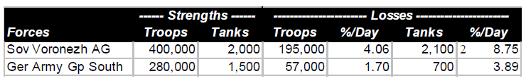
A comparison of forces and losses of the Soviet Voronezh Army Group and German Army Group South on the south face of the Kursk Salient is shown below. The strengths are averages over the 12 days of the battle, taking into consideration initial strengths, losses, and reinforcements.
A comparison of the casualty tradeoff can be found by dividing Soviet casualties by German strength, and German losses by Soviet strength. On that basis, 100 Germans inflicted 5.8 casualties per day on the Soviets, while 100 Soviets inflicted 1.2 casualties per day on the Germans, a tradeoff of 4.9 to 1.0
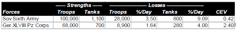
The statistics for the 8-day offensive of the German XLVIII Panzer Corps toward Oboyan are shown below. Also shown is the relative combat effectiveness value (CEV) of Germans and Soviets, as calculated by the TNDM. As was the case for the Battle of Antietam, this is derived from a mathematical comparison of the theoretical combat power ratio of the two forces (simply considering numbers and weapons characteristics), and the actual combat power ratios reflected by the battle results:
The calculated CEVs suggest that 100 German troops were the combat equivalent of 240 Soviet troops, comparably equipped. The casualty tradeoff in this battle shows that 100 Germans inflicted 5.15 casualties per day on the Soviets, while 100 Soviets inflicted 1.11 casualties per day on the Germans, a tradeoff of4.64. It is a rule of thumb that the casualty tradeoff is usually about the square of the CEV.
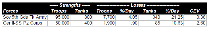
A similar comparison can be made of the two-day battle of Prokhorovka. Soviet accounts of that battle have claimed this as a great victory by the Soviet Fifth Guards Tank Army over the German II SS Panzer Corps. In fact, since the German advance was halted, the outcome was close to a draw, but with the advantage clearly in favor of the Germans.
The casualty tradeoff shows that 100 Germans inflicted 7.7 casualties per on the Soviets, while 100 Soviets inflicted 1.0 casualties per day on the Germans, for a tradeoff value of 7.7.
When the German offensive began, they had a slight degree of local air superiority. This was soon reversed by German and Soviet shifts of air elements, and during most of the offensive, the Soviets had a slender margin of air superiority. In terms of technology, the Germans probably had a slight overall advantage. However, the Soviets had more tanks and, furthermore, their T-34 was superior to any tank the Germans had available at the time. The CEV calculations demonstrate that the Germans had a great qualitative superiority over the Russians, despite near-equality in technology, and despite Soviet air superiority. The Germans lost the battle, but only because they were overwhelmed by Soviet numbers.
German Performance, Western Europe, 1943-1945
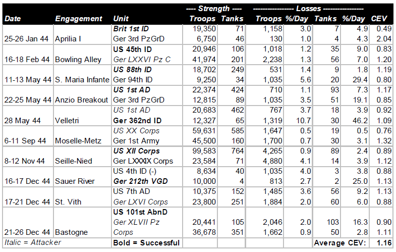
Beginning with operations between Salerno and Naples in September, 1943, through engagements in the closing days of the Battle of the Bulge in January, 1945, the pattern of German performance against the Western Allies was consistent. Some German units were better than others, and a few Allied units were as good as the best of the Germans. But on the average, German performance, as measured by CEV and casualty tradeoff, was better than the Western allies by a CEV factor averaging about 1.2, and a casualty tradeoff factor averaging about 1.5. Listed below are ten engagements from Italy and Northwest Europe during that 1944.
Technologically, German forces and those of the Western Allies were comparable. The Germans had a higher proportion of armored combat vehicles, and their best tanks were considerably better than the best American and British tanks, but the advantages were at least offset by the greater quantity of Allied armor, and greater sophistication of much of the Allied equipment. The Allies were increasingly able to achieve and maintain air superiority during this period of slightly less than two years.
The combination of vast superiority in numbers of troops and equipment, and in increasing Allied air superiority, enabled the Allies to fight their way slowly up the Italian boot, and between June and December, 1944, to drive from the Normandy beaches to the frontier of Germany. Yet the presence or absence of Allied air support made little difference in terms of either CEVs or casualty tradeoff values. Despite the defeats inflicted on them by the numerically superior Allies during the latter part of 1944, in December the Germans were able to mount a major offensive that nearly destroyed an American army corps, and threatened to drive at least a portion of the Allied armies into the sea.
Clearly, in their battles against the Soviets and the Western Allies, the Germans demonstrated that quality of combat troops was able consistently to overcome Allied technological and air superiority. It was Allied numbers, not technology, that defeated the quantitatively superior Germans.
The Six-Day War, 1967
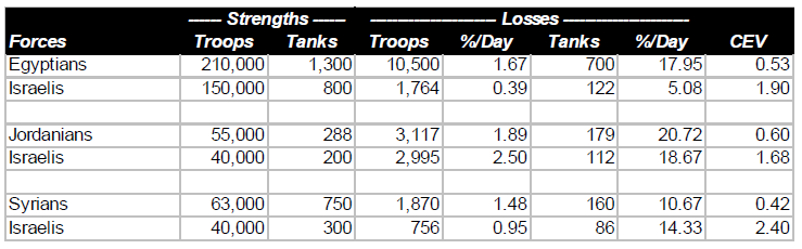
The remarkable Israeli victories over far more numerous Arab opponents—Egyptian, Jordanian, and Syrian—in June, 1967 revealed an Israeli combat superiority that had not been suspected in the United States, the Soviet Union or Western Europe. This superiority was equally awesome on the ground as in the air. (By beginning the war with a surprise attack which almost wiped out the Egyptian Air Force, the Israelis avoided a serious contest with the one Arab air force large enough, and possibly effective enough, to challenge them.) The results of the three brief campaigns are summarized in the table below:
It should be noted that some Israelis who fought against the Egyptians and Jordanians also fought against the Syrians. Thus, the overall Arab numerical superiority was greater than would be suggested by adding the above strength figures, and was approximately 328,000 to 200,000.
It should also be noted that the technological sophistication of the Israeli and Arab ground forces was comparable. The only significant technological advantage of the Israelis was their unchallenged command of the air. (In terms of battle outcomes, it was irrelevant how they had achieved air superiority.) In fact this was a very significant advantage, the full import of which would not be realized until the next Arab-Israeli war.
The results of the Six Day War do not provide an unequivocal basis for determining the relative importance of human factors and technological superiority (as evidenced in the air). Clearly a major factor in the Israeli victories was the superior performance of their ground forces due mainly to human factors. At least as important in those victories was Israeli command of the air, in which both technology and human factors both played a part.
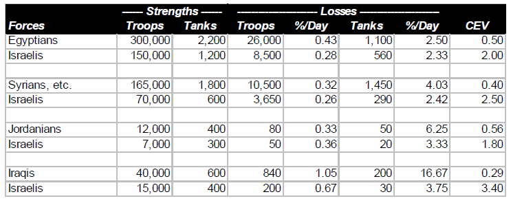
The October War, 1973
A better basis for comparing the relative importance of human factors and technology is provided by the results of the October War of 1973 (known to Arabs as the War of Ramadan, and to Israelis as the Yom Kippur War). In this war the Israeli unquestioned superiority in the air was largely offset by the Arabs possession of highly sophisticated Soviet air defense weapons.
One important lesson of this war was a reassessment of Israeli contempt for the fighting quality of Arab ground forces (which had stemmed from the ease with which they had won their ground victories in 1967). When Arab ground troops were protected from Israeli air superiority by their air defense weapons, they fought well and bravely, demonstrating that Israeli control of the air had been even more significant in 1967 than anyone had then recognized.
It should be noted that the total Arab (and Israeli) forces are those shown in the first two comparisons, above. A Jordanian brigade and two Iraqi divisions formed relatively minor elements of the forces under Syrian command (although their presence on the ground was significant in enabling the Syrians to maintain a defensive line when the Israelis threatened a breakthrough around 20 October). For the comparison of Jordanians and Iraqis the total strength is the total of the forces in the battles (two each) on which these comparisons are based.
One other thing to note is how the Israelis, possibly unconsciously, confirmed that validity of their CEVs with respect to Egyptians and Syrians by the numerical strengths of their deployments to the two fronts. Since the war ended up in a virtual stalemate on both fronts, the overall strength figures suggest rough equivalence of combat capability.
The CEV values shown in the above table are very significant in relation to the debate about human factors and technology, There was little if anything to choose between the technological sophistication of the two sides. The Arabs had more tanks than the Israelis, but (as Israeli General Avraham Adan once told the author) there was little difference in the quality of the tanks. The Israelis again had command of the air, but this was neutralized immediately over the battlefields by the Soviet air defense equipment effectively manned by the Arabs. Thus, while technology was of the utmost importance to both sides, enabling each side to prevent the enemy from gaining a significant advantage, the true determinant of battlefield outcomes was the fighting quality of the troops, And, while the Arabs fought bravely, the Israelis fought much more effectively. Human factors made the difference.
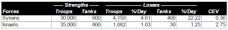
Israeli Invasion of Lebanon, 1982
In terms of the debate about the relative importance of human factors and technology, there are two significant aspects to this small war, in which Syrians forces and PLO guerrillas were the Arab participants. In the first place, the Israelis showed that their air technology was superior to the Syrian air defense technology, As a result, they regained complete control of the skies over the battlefields. Secondly, it provides an opportunity to include a highly relevant quotation.
The statistical comparison shows the results of the two major battles fought between Syrians and Israelis:
In assessing the above statistics, a quotation from the Israeli Chief of Staff, General Rafael Eytan, is relevant.
In late 1982 a group of retired American generals visited Israel and the battlefields in Lebanon. Just before they left for home, they had a meeting with General Eytan. One of the American generals asked Eytan the following question: “Since the Syrians were equipped with Soviet weapons, and your troops were equipped with American (or American-type) weapons, isn’t the overwhelming Israeli victory an indication of the superiority of American weapons technology over Soviet weapons technology?”
Eytan’s reply was classic: “If we had had their weapons, and they had had ours, the result would have been absolutely the same.”
One need not question how the Israeli Chief of Staff assessed the relative importance of the technology and human factors.
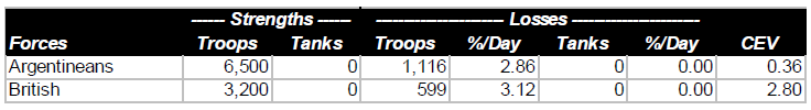
Falkland Islands War, 1982
It is difficult to get reliable data on the Falkland Islands War of 1982. Furthermore, the author of this article had not undertaken the kind of detailed analysis of such data as is available. However, it is evident from the information that is available about that war that its results were consistent with those of the other examples examined in this article.
The total strength of Argentine forces in the Falklands at the time of the British counter-invasion was slightly more than 13,000. The British appear to have landed close to 6,400 troops, although it may have been fewer. In any event, it is evident that not more than 50% of the total forces available to both sides were actually committed to battle. The Argentine surrender came 27 days after the British landings, but there were probably no more than six days of actual combat. During these battles the British performed admirably, the Argentinians performed miserably. (Save for their Air Force, which seems to have fought with considerable gallantry and effectiveness, at the extreme limit of its range.) The British CEV in ground combat was probably between 2.5 and 4.0. The statistics were at least close to those presented below:
It is evident from published sources that the British had no technological advantage over the Argentinians; thus the one-sided results of the ground battles were due entirely to British skill (derived from training and doctrine) and determination.
South African Operations in Angola, 1987-1988
Neither the political reasons for, nor political results of, the South African military interventions in Angola in the 1970s, and again in the late 1980s, need concern us in our consideration of the relative significance of technology and of human factors. The combat results of those interventions, particularly in 1987-1988 are, however, very relevant.
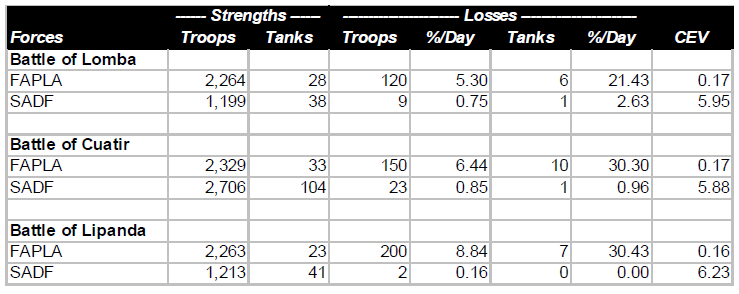
The operations between elements of the South African Defense Force (SADF) and forces of the Popular Movement for the Liberation of Angola (FAPLA) took place in southeast Angola, generally in the region east of the city of Cuito-Cuanavale. Operating with the SADF units were a few small units of Jonas Savimbi’s National Union for the Total Independence of Angola (UNITA). To provide air support to the SADF and UNITA ground forces, it would have been necessary for the South Africans to establish air bases either in Botswana, Southwest Africa (Namibia), or in Angola itself. For reasons that were largely political, they decided not to do that, and thus operated under conditions of FAPLA air supremacy. This led them, despite terrain generally unsuited for armored warfare, to use a high proportion of armored vehicles (mostly light armored cars) to provide their ground troops with some protection from air attack.
Summarized below are the results of three battles east of Cuito-Cuanavale in late 1987 and early 1988. Included with FAPLA forces are a few Cubans (mostly in armored units); included with the SADF forces are a few UNITA units (all infantry).
FAPLA had complete command of air, and substantial numbers of MiG-21 and MiG-23 sorties were flown against the South Africans in all of these battles. This technological superiority was probably partly offset by greater South African EW (electronic warfare) capability. The ability of the South Africans to operate effectively despite hostile air superiority was reminiscent of that of the Germans in World War II. It was a further demonstration that, no matter how important technology may be, the fighting quality of the troops is even more important.
The tank figures include armored cars. In the first of the three battles considered, FAPLA had by far the more powerful and more numerous medium tanks (20 to 0). In the other two, SADF had a slight or significant advantage in medium tank numbers and quality. But it didn’t seem to make much difference in the outcomes.
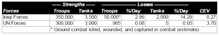
Kuwait War, 1991
The previous seven examples permit us to examine the results of Kuwait (or Second Gulf) War with more objectivity than might otherwise have possible. First, let’s look at the statistics. Note that the comparison shown below is for four days of ground combat, February 24-28, and shows only operations of U.S. forces against the Iraqis.
There can be no question that the single most important contribution to the overwhelming victory of U.S. and other U.N. forces was the air war that preceded, and accompanied, the ground operations. But two comments are in order. The air war alone could not have forced the Iraqis to surrender. On the other hand, it is evident that, even without the air war, U.S. forces would have readily overwhelmed the Iraqis, probably in more than four days, and with more than 285 casualties. But the outcome would have been hardly less one-sided.
The Vietnam War, 1965-1973
It is impossible to make the kind of mathematical analysis for the Vietnam War as has been done in the examples considered above. The reason is that we don’t have any good data on the Vietcong—North Vietnamese forces,
However, such quantitative analysis really isn’t necessary There can be no doubt that one of the opponents was a superpower, the most technologically advanced nation on earth, while the other side was what Lyndon Johnson called a “raggedy-ass little nation,” a typical representative of “the third world.“
Furthermore, even if we were able to make the analyses, they would very possibly be misinterpreted. It can be argued (possibly with some exaggeration) that the Americans won all of the battles. The detailed engagement analyses could only confirm this fact. Yet it is unquestionable that the United States, despite airpower and all other manifestations of technological superiority, lost the war. The human factor—as represented by the quality of American political (and to a lesser extent military) leadership on the one side, and the determination of the North Vietnamese on the other side—was responsible for this defeat.
Conclusion
In a recent article in the Armed Forces Journal International Col. Philip S. Neilinger, USAF, wrote: “Military operations are extremely difficult, if not impossible, for the side that doesn’t control the sky.” From what we have seen, this is only partly true. And while there can be no question that operations will always be difficult to some extent for the side that doesn’t control the sky, the degree of difficulty depends to a great degree upon the training and determination of the troops.
What we have seen above also enables us to view with a better perspective Colonel Neilinger’s subsequent quote from British Field Marshal Montgomery: “If we lose the war in the air, we lose the war and we lose it quickly.” That statement was true for Montgomery, and for the Allied troops in World War II. But it was emphatically not true for the Germans.
The examples we have seen from relatively recent wars, therefore, enable us to establish priorities on assuring readiness for war. It is without question important for us to equip our troops with weapons and other materiel which can match, or come close to matching, the technological quality of the opposition’s materiel. We must realize that we cannot—as some people seem to think—buy good forces, by technology alone. Even more important is to assure the fighting quality of the troops. That must be, by far, our first priority in peacetime budgets and in peacetime military activities of all sorts.
NOTES
[1] This calculation is automatic in analyses of historical battles by the Tactical Numerical Deterministic Model (TNDM).
[2] The initial tank strength of the Voronezh Army Group was about 1,100 tanks. About 3,000 additional Soviet tanks joined the battle between 6 and 12 July. At the end of the battle there were about 1,800 Soviet tanks operational in the battle area; at the same time there were about 1,000 German tanks still operational.
[3] The relative combat effectiveness value of each force is calculated in comparison to 1.0. Thus the CEV of the Germans is 2.40:1.0, while that of the Soviets is 0.42: 1.0. The opposing CEVs are always the reciprocals of each other.
The first was chosen to provide a historical context for the 3:1 rule of thumb. The second was chosen so as to examine how this rule applies to modern combat data.
We decided that this should be tested to the RAND version of the 3:1 rule as documented by RAND in 1992 and used in JICM [Joint Integrated Contingency Model] (with SFS [Situational Force Scoring]) and other models. This rule, as presented by RAND, states: “[T]he famous ‘3:1 rule,’ according to which the attacker and defender suffer equal fractional loss rates at a 3:1 force ratio if the battle is in mixed terrain and the defender enjoys ‘prepared’ defenses…”
Therefore, we selected out all those engagements from these two databases that ranged from force ratios of 2.5 to 1 to 3.5 to 1 (inclusive). It was then a simple matter to map those to a chart that looked at attackers losses compared to defender losses. In the case of the pre-1904 cases, even with a large database (243 cases), there were only 12 cases of combat in that range, hardly statistically significant. That was because most of the combat was at odds ratios in the range of .50-to-1 to 2.00-to-one.
The count of number of engagements by odds in the pre-1904 cases:
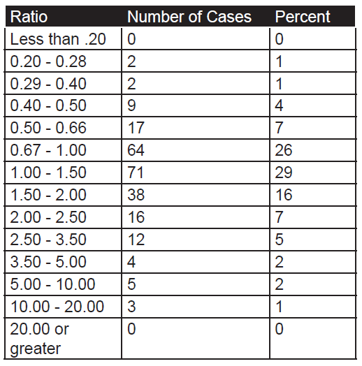
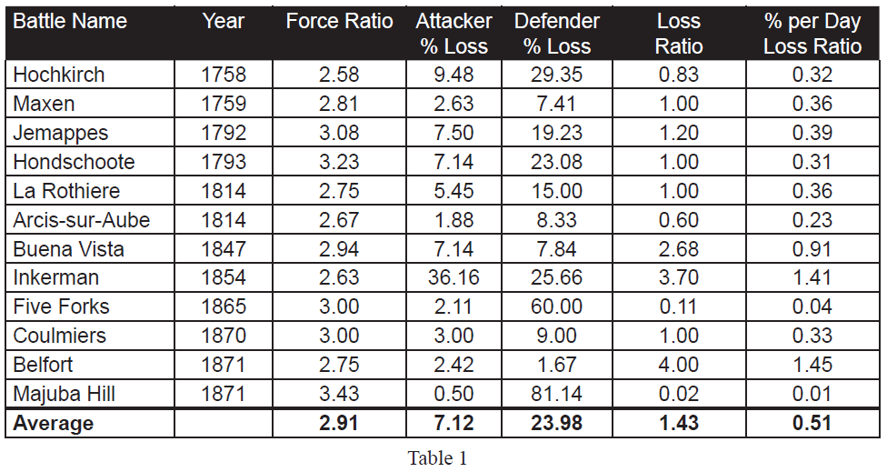
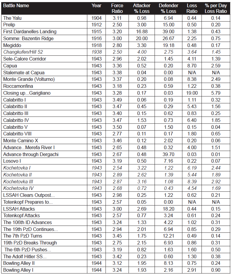
As the database is one of battles, then usually these are only joined at reasonably favorable odds, as shown by the fact that 88 percent of the battles occur between 0.40 and 2.50 to 1 odds. The twelve pre-1904 cases in the range of 2.50 to 3.50 are shown in Table 1.
If the RAND version of the 3:1 rule was valid, one would expect that the “Percent per Day Loss Ratio” (the last column) would hover around 1.00, as this is the ratio of attacker percent loss rate to the defender percent loss rate. As it is, 9 of the 12 data points are noticeably below 1 (below 0.40 or a 1 to 2.50 exchange rate). This leaves only three cases (25%) with an exchange rate that would support such a “rule.”
If we look at the simple ratio of actual losses (vice percent losses), then the numbers comes much closer to parity, but this is not the RAND interpretation of the 3:1 rule. Six of the twelve numbers “hover” around an even exchange ratio, with six other sets of data being widely off that central point. “Hover” for the rest of this discussion means that the exchange ratio ranges from 0.50-to-1 to 2.00-to 1.
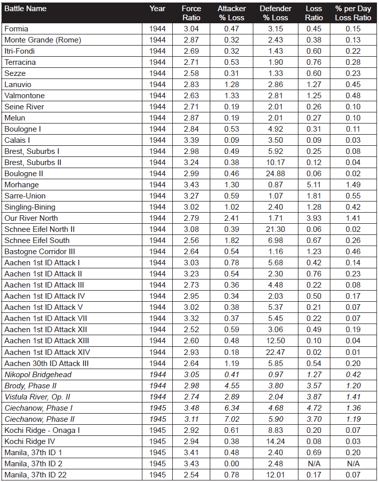
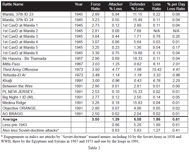
Still, this is early modern linear combat, and is not always representative of modern war. Instead, we will examine 634 cases in the Division-level Database (which consists of 675 cases) where we have worked out the force ratios. While this database covers from 1904 to 1991, most of the cases are from WWII (1939- 1945). Just to compare:
As such, 87% of the cases are from WWII data and 10% of the cases are from post-WWII data. The engagements without force ratios are those that we are still working on as The Dupuy Institute is always expanding the DLEDB as a matter of routine. The specific cases, where the force ratios are between 2.50 and 3.50 to 1 (inclusive) are shown in Table 2:
This is a total of 98 engagements at force ratios of 2.50 to 3.50 to 1. It is 15 percent of the 634 engagements for which we had force ratios. With this fairly significant representation of the overall population, we are still getting no indication that the 3:1 rule, as RAND postulates it applies to casualties, does indeed fit the data at all. Of the 98 engagements, only 19 of them demonstrate a percent per day loss ratio (casualty exchange ratio) between 0.50-to-1 and 2-to-1. This is only 19 percent of the engagements at roughly 3:1 force ratio. There were 72 percent (71 cases) of those engagements at lower figures (below 0.50-to-1) and only 8 percent (cases) are at a higher exchange ratio. The data clearly was not clustered around the area from 0.50-to- 1 to 2-to-1 range, but was well to the left (lower) of it.
Looking just at straight exchange ratios, we do get a better fit, with 31 percent (30 cases) of the figure ranging between 0.50 to 1 and 2 to 1. Still, this figure exchange might not be the norm with 45 percent (44 cases) lower and 24 percent (24 cases) higher. By definition, this fit is 1/3rd the losses for the attacker as postulated in the RAND version of the 3:1 rule. This is effectively an order of magnitude difference, and it clearly does not represent the norm or the center case.
The percent per day loss exchange ratio ranges from 0.00 to 5.71. The data tends to be clustered at the lower values, so the high values are very much outliers. The highest percent exchange ratio is 5.71, the second highest is 4.41, the third highest is 2.92. At the other end of the spectrum, there are four cases where no losses were suffered by one side and seven where the exchange ratio was .01 or less. Ignoring the “N/A” (no losses suffered by one side) and the two high “outliers (5.71 and 4.41), leaves a range of values from 0.00 to 2.92 across 92 cases. With an even distribution across that range, one would expect that 51 percent of them would be in the range of 0.50-to-1 and 2.00-to-1. With only 19 percent of the cases being in that range, one is left to conclude that there is no clear correlation here. In fact, it clearly is the opposite effect, which is that there is a negative relationship. Not only is the RAND construct unsupported, it is clearly and soundly contradicted with this data. Furthermore, the RAND construct is theoretically a worse predictor of casualty rates than if one randomly selected a value for the percentile exchange rates between the range of 0 and 2.92. We do believe this data is appropriate and accurate for such a test.
As there are only 19 cases of 3:1 attacks falling in the even percentile exchange rate range, then we should probably look at these cases for a moment:
One will note, in these 19 cases, that the average attacker casualties are way out of line with the average for the entire data set (3.20 versus 1.39 or 3.20 versus 0.63 with pre-1943 and Soviet-doctrine attackers removed). The reverse is the case for the defenders (3.12 versus 6.08 or 3.12 versus 5.83 with pre-1943 and Soviet-doctrine attackers removed). Of course, of the 19 cases, 2 are pre-1943 cases and 7 are cases of Soviet-doctrine attackers (in fact, 8 of the 14 cases of the Soviet-doctrine attackers are in this selection of 19 cases). This leaves 10 other cases from the Mediterranean and ETO (Northwest Europe 1944). These are clearly the unusual cases, outliers, etc. While the RAND 3:1 rule may be applicable for the Soviet-doctrine offensives (as it applies to 8 of the 14 such cases we have), it does not appear to be applicable to anything else. By the same token, it also does not appear to apply to virtually any cases of post-WWII combat. This all strongly argues that not only is the RAND construct not proven, but it is indeed clearly not correct.
The fact that this construct also appears in Soviet literature, but nowhere else in US literature, indicates that this is indeed where the rule was drawn from. One must consider the original scenarios run for the RSAC [RAND Strategy Assessment Center] wargame were “Fulda Gap” and Korean War scenarios. As such, they were regularly conducting battles with Soviet attackers versus Allied defenders. It would appear that the 3:1 rule that they used more closely reflected the experiences of the Soviet attackers in WWII than anything else. Therefore, it may have been a fine representation for those scenarios as long as there was no US counterattacking or US offensives (and assuming that the Soviet Army of the 1980s performed at the same level as in did in the 1940s).
There was a clear relative performance difference between the Soviet Army and the German Army in World War II (see our Capture Rate Study Phase I & II and Measuring Human Factors in Combat for a detailed analysis of this).[1] It was roughly in the order of a 3-to-1-casualty exchange ratio. Therefore, it is not surprising that Soviet writers would create analytical tables based upon an equal percentage exchange of losses when attacking at 3:1. What is surprising, is that such a table would be used in the US to represent US forces now. This is clearly not a correct application.
Therefore, RAND’s SFS, as currently constructed, is calibrated to, and should only be used to represent, a Soviet-doctrine attack on first world forces where the Soviet-style attacker is clearly not properly trained and where the degree of performance difference is similar to that between the Germans and Soviets in 1942-44. It should not be used for US counterattacks, US attacks, or for any forces of roughly comparable ability (regardless of whether Soviet-style doctrine or not). Furthermore, it should not be used for US attacks against forces of inferior training, motivation and cohesiveness. If it is, then any such tables should be expected to produce incorrect results, with attacker losses being far too high relative to the defender. In effect, the tables unrealistically penalize the attacker.
As JICM with SFS is now being used for a wide variety of scenarios, then it should not be used at all until this fundamental error is corrected, even if that use is only for training. With combat tables keyed to a result that is clearly off by an order of magnitude, then the danger of negative training is high.
Christopher A. Lawrence, War by Numbers: Understanding Conventional Combat (Lincoln, NE: Potomac Books, 2017) 390 pages, $39.95
War by Numbers assesses the nature of conventional warfare through the analysis of historical combat. Christopher A. Lawrence (President and Executive Director of The Dupuy Institute) establishes what we know about conventional combat and why we know it. By demonstrating the impact a variety of factors have on combat he moves such analysis beyond the work of Carl von Clausewitz and into modern data and interpretation.
Using vast data sets, Lawrence examines force ratios, the human factor in case studies from World War II and beyond, the combat value of superior situational awareness, and the effects of dispersion, among other elements. Lawrence challenges existing interpretations of conventional warfare and shows how such combat should be conducted in the future, simultaneously broadening our understanding of what it means to fight wars by the numbers.
The book is available in paperback directly from Potomac Books and in paperback and Kindle from Amazon.
Informal portrait of Charles E. W. Bean working on official files in his Victoria Barracks office during the writing of the Official History of Australia in the War of 1914-1918. The files on his desk are probably the Operations Files, 1914-18 War, that were prepared by the army between 1925 and 1930 and are now held by the Australian War Memorial as AWM 26. Courtesy of the Australian War Memorial. [Defence in Depth]
Although the posts are a couple of years old now, Dr. Robert T. Foley of the Defence Studies Department at King’s College London has provided a wonderful compilation of links to digital holdings and resources documenting the experiences of many of the many belligerents in the First World War. The links include digitized archival holdings and electronic copies of often hard-to-find official histories of ground, sea, and air operations.
For TDI, the availability of such materials greatly broadens potential sources for research on historical combat. For example, TDI made use of German regional archival holdings for to compile data on the use of chemical weapons in urban environments from the separate state armies that formed part of the Imperial German Army in the First World War. Although much of the German Army’s historical archives were destroyed by Allied bombing at the end of the Second World War, a great deal of material survived in regional state archives and in other places, as Dr. Foley shows. Access to the highly detailed official histories is another boon for such research.
The Digital Era hints at unprecedented access to historical resources and more materials are being added all the time. Current historians should benefit greatly. Future historians, alas, are not as likely to be so fortunate when it comes time to craft histories of the the current era.