I have four books in process or about to be released. They are:
The Battle for Kyiv:
– UK release date: 28 November
– U.S. release date: 18 January 2024
Aces at Kursk:
– UK release date: 30 January 2024
– U.S. release date: posted as 18 January 2024, but suspect release date will be in March 2024.
Hunting Falcon:
– UK release date: 28 February 2024
– U.S. release date: posted as 29 February 2024, but suspect released date will be in April 2024.
The Siege of Mariupol:
– UK release date: sometime in 2024
– U.S. release date: sometime in 2024
Books under consideration for 2024/2025:
– The Battle for the Donbas
– The Battle of Tolstoye Woods (from the Battle of Kursk)
– More War by Numbers
The Dupuy Institute
Excellence in Historical Research and Analysis
The Dupuy Institute
Excellence in Historical Research and Analysis
Category Land Warfare
Video of Infantry Fighting near Bakhmut
This video has been floating around for a few days. It is worth watching. More 1916 than RMA. This is fighting outside of Bakhmut on the route into the town. There are pictures of people being shot in this video.
A few observations:
- 0:44: One Ukranian soldier has been killed “Norman.”
- 1:08: Grenade attack?
- 1:30: first JRR Tolkien reference.
- 1:37: second JRR Tolkien reference.
- 1:56: grenade being thrown.
- 2:30: three clear targets
- 2:40: clip change
- 2:50: shooting continues
- 3:34: Another Tolkien reference.
- 3:38: Other people deployed
- I see that three Russians have been killed so far. Looks like all were done by one man, “Tikhey”
- 5:35: instructions to preserve ammo.
- 5:38: wounded Russian
- 6:24: Another clip change
- 6:31: incoming mortar fire
- 7:14: Two more Russians engaged.
- 7:44: It is claimed Russian is killed.
- 9:02: Close in mortar hit
- 10:10: One person is reported wounded.
- 10:26: “Normans” magazines have been used.
These are the Da Vinci Wolves: Da Vinci Wolves | MilitaryLand.net. The “Right Sector” is a far-right Ukrainian nationalist organization (see: Right Sector – Wikipedia). They currently hold no seats in the Ukrainian parlament (the Rada).
Other similar videos:
Ukrainian soldiers take Russian trench in terrifying POV footage from Bakhmut – YouTube
First video as annotated by The Telegraph: Ukrainian soldiers fight off Russians in battle for Bakhmut – ‘Orcs jumped into our trenches’ – YouTube
Advance Rates in Combat
Advance Rates in Combat:
Units maneuver before and during a battle to achieve a more favorable position. This maneuver is often unopposed and is not the subject of this discussion. Unopposed movement before combat is often quite fast, although often not as fast as people would like to assume. Once engaged with an opposing force, the front line between them also moves, usually moving forwards if the attacker is winning and moving backwards for the defender if he is losing or choosing to withdraw. These are opposed advance rates. This section is focused on discussing opposed advance rates or “advance rates in combat.”
The operations research and combat modeling community have often taken a short-hand step of predicting advance rates in combat based upon force ratios, so that a force with a three-to-one force ratio advances faster than a force with a two-to-one force ratio. But, there is not a direct relationship between force ratios and advance rates. There is an indirect relationship between them, in that higher forces ratios increased the chances of winning, and winning the combat and the degree of victory helps increase advance rates. There is little analytical work that has been done on this subject.[1]
Opposed advance rates are very much influenced by 1) terrain, 2) weather and 3) the degree of mechanization and mobilization, in addition to 4) the degree of enemy opposition. These four factors all influence what the rates will be.
In a study The Dupuy Institute did on enemy prisoner of war capture rates, we ended up coding a series of engagements by outcome. This has proven to a useful coding for the examination of advance rates. Engagements codes as outcomes I and II (limited action and limited attack) are not of concern for this discussion. The engagement coded as attack fails (outcome III) is significant, as these are cases where the attacker is determined to have failed. As such they often do not advance at all, sometimes have a very limited advance and sometimes are even pushed back (have a negative advance). For example, in our work on the subject, of our 271 division-level engagements from Western Europe 1943-45 the average advance rate was 1.81 kilometers per day. For Eastern Europe in 1943 the average advance rate was 4.54 kilometers per day based upon 173 division-level engagements.[2] These advance rates are irrespective of what the force ratios are for an engagement.
In contrast, in those engagements where the attacker is determined to have won and is coded as attacker advances (outcome IV) the attacker advances an average of 2.00 kilometers in the 142 engagements from Western Europe 1943-45. The average force ratio of these engagements was 2.17. In the case of Eastern Europe in 1943, the average advance rate was 5.80 kilometers based upon 73 engagements. The average force ratio of these engagements was 1.62.
We also coded engagements where the defender was penetrated (outcome V). These are those cases where the attacker penetrated the main defensive line of the defending unit, forcing them to either withdraw, reposition or counterattack. This penetration is achieved by either overwhelming combat power, the end result of an extended operation that finally pushes through the defenses, or a gap in the defensive line usually as a result of a mistake. Superior mechanization or mobility for the attacker can also make a difference. In those engagements where the defender was determined to have been penetrated the attacker advanced an average of 4.12 kilometers in 34 engagements from Western Europe 1943-45. The average force ratio of these engagements was 2.31. In the case of Eastern Europe in 1943, the average advance rates was 11.28 kilometers based upon 19 engagements. The average force ratio of these engagements was 1.99.
This clearly shows the difference in advance rate based upon outcome. It is only related to force ratios to the extant the force ratios are related to producing these different outcomes.
Also of significance is terrain and weather. Needless to say, significant blocking obstacles like bodies of water, can halt an advance and various rivers and creeks often considerably slow them, even with engineering and bridging support. Rugged terrain is more difficult to advance through and easier to defend and delay then smoother terrain. Closed or wooded terrain is more difficult to advance through and easier to defend and delay then open terrain. Urban terrain tends to also slow down advance rates, being effectively “closed terrain.” If it is raining then advance rates are slower than in clear weather. Sometimes considerably slower in heavy rain. The season it is, which does influence the amount of daylight, also affects the advance rate. Units move faster in daylight than in darkness. This is all heavily influenced by the road network and the number of roads in the area of advance.
No systematic study of advance rates has been done by the operations research community. Probably the most developed discussion of the subject was the material assembled for the combat models developed by Trevor Dupuy. This included addressing the effects of terrain and weather and road network on the advance rates. A combat model is an imperfect theory of combat.
Even though this combat modeling effort is far from perfect and fundamentally based upon quantifying factors derived by professional judgment, tables derived from this modeling effort have become standard presentations in a couple of U.S. Army and USMC planning and reference manuals. This includes U.S. Army Staff Reference Guide and the Marine Corps’ MAGTF Planner’s Reference Manual.[3]
The original table, from Numbers, Predictions and War, is here:[4]
STANDARD (UNMODIFIED) ADVANCE RATES
Rates in km/day
Armored Mechzd. Infantry Horse Cavalry
Division Division Division Division or
or Force Force
Against Intense Resistance
(P/P: 1.0-1.1O)
Hasty defense/delay 4.0 4.0 4.0 3.0
Prepared defense 2.0 2.0 2.0 1.6
Fortified defense 1.0 1.0 1.0 0.6
Against Strong/Intense Resistance
(P/P: 1-11-125)
Hasty defense/delay 5.0 4.5 4.5 3.5
Prepared defense 2.25 2.25 2.25 1.5
Fortified defense 1.25 1.25 1.25 0.7
Against Strong Defense
(P/P: 1.26-1.45)
Hasty defense/delay 6.0 5.0 5.0 4.0
Prepared defense 2.5 2.5 2.5 2.0
Fortified defense 1.5 1.5 1.5 0.8
Against Moderate/Strong Resistance
(P/P: 1.46-1.75)
Hasty defense 9.0 7.5 6.5 6.0
Prepared defense 4.0 3.5 3.0 2.5
Fortified defense 2.0 2.0 1.75 0.9
Against Moderate Resistance
(P/P: 1.76-225)
Hasty defense/delay 12.0 10.0 8.0 8.0
Prepared defense 6.0 5.0 4.0 3.0
Fortified defense 3.0 2.5 2.0 1.0
Against Slight/Moderate Resistance
(P/P:2.26-3.0)
Hasty defense/delay 16.0 13.0 10.0 12.0
Prepared defense 8.0 7.0 5.0 6.0
Fortified defense 4.0 3.0 2.5 2.0
Against Slight Resistance
(P/P: 3.01-4.25)
Hasty defense/delay 20.0 16.0 12.0 15.0
Prepared defense 10.0 8.0 6.0 7.0
Fortified defense 5.0 4.0 3.0 4.0
Against Negligible/Slight Resistance
(P/P:4.26-6.00)
Hasty defense/delay 40.0 30.0 18.0 28.0
Prepared defense 20.0 16.0 10.0 14.0
Fortified defense 10.0 8.0 6.0 7.0
Against Negligible Resistance
(P/P: 6.00 plus)
Hasty defense /delay 60.0 48.0 24.0 40.0
Prepared/fortified defense 30.0 24.0 12.0 12.0
*Based on HERO studies: ORALFORE, Barrier Effectiveness, and Combat Data Subscription Service.
** For armored and mechanized infantry divisions, these rates can be sustained for 10 days only; for the next 20 days standard rates for armored and mechanized infantry forces cannot exceed half these rates.
This is a modeling construct built from historical data. These are “unmodified” rates. The modifications include: 1) General Terrain Factors (ranging from 0.4 to 1.05 for Infantry (combined arms) Force and from 0.2 to 1.0 for Cavalry or Armored Force, 2) Road Quality Factors (addressing Road Quality from 0.6 to 1.0 and Road Density from 0.6 to 1.0), 3) Obstacles Factors (ranging from 0.5 to 0.9 for both a River or steam and for Minefields), 4) Day/Night with night advance rate one-half of daytime advance rate and 5) Main Effort Factor (ranging from 1.0 to 1.2). These last five sets of tables are not shown here, but can be found in his writings.[5]
[1] The most significant works we are aware of is Trevor Dupuy’s ORALFORE study in 1972: Opposed Rates of Advance in Large Forces in Europe (ORALFORE), (TNDA, for DCSOPS, 1972); Trevor Dupuy’s 1979 book Numbers, Predictions and War; and a series of three papers by Robert Helmbold (Center for Army Analysis): “Rates of Advance in Land Combat Operations, June 1990,” “Survey of Past Work on Rates of Advance, and “A Compilation of Data on Rates of Advance.”
[2] See paper on the subject by Christopher A. Lawrence, “Advance Rates in Combat based upon Outcome,” posted on the blog Mystics & Statistic, April 2023. In the databases, there were 282 Western Europe engagements from September 1943 to January 1945. There were 256 Eastern Front engagements from February, March, July and August of 1943.
[3] See U.S. Army Staff Reference Guide, Volume I: Unclassified Resources, December 2020, ATP 5-0.2-1, pages xi and 220; and MAGTF Planner’s Reference Manual, MSTF pamphlet 5-0.3, October 2010, page 79. Both manuals include a table for division-level advances which is derived from Trevor Dupuy’s work, and both manuals contain a table for brigade-level and below advances which are calculated per hour that appear to also be derived from Trevor Dupuy’s division-level table. The U.S. Army manual gives the “brigade and below” advance rates in km/hr while the USMC manual, which appears to be the same table, gives the “brigade and below” advance rates in km/day. This appears to be a typo.
[4] Numbers, Predictions and War, pages 213-214. The sixth line of numbers, three numbers were changes from 1.85 to 1.25 as this was obviously a typo in the original.
[5] See Numbers, Predictions and War, pages 214-216.
The actual paper this was drawn from is here: Advance Rates in Combat
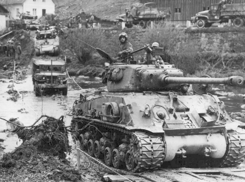
American Thunder: U.S. Army Tank Design, Development and Doctrine in World War II
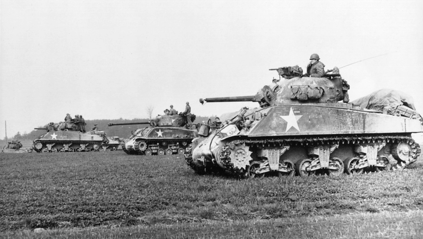
Just to give you a heads up, Richard Anderson, former researcher at TDI, is publishing the book American Thunder as of December 16, 2023. It will make for a great stocking stuffer for the right person. See: Amazon.com: American Thunder: U.S. Army Tank Design, Development, and Doctrine in World War II: 9780811773812: Anderson, Richard: Books. This is his fourth book (American Thunder, Cracking Hitler’s Atlantic Wall, Artillery Hell, Hitler’s Last Gamble). He has been working on this last one for over fourteen years.
The table of contents are:
Introduction 1
Acknowledgements 4
U.S. Army World War II Procurement and Nomenclature 6
Part One: Organization, Development, and Production from Armistice Day to VJ Day 13
Chapter 1 Stagnation and Rebirth: The Lean Years from the End of the Great War to 1 September 1939 14
Chapter 2 State of the Art: The View Looking in, Sereno Brett and Arthur Hadsell 62
Chapter 3 Learning to Walk: 1 September 1939 to 30 June 1940 73
Chapter 4 State of the Art: The View Looking Out, the Spanish Civil War 94
Chapter 5 The Sleeping Giant Stirs: 1 July to 31 December 1940 107
Chapter 6 The Threat Perceived 129
Chapter 7 Explosive Growth…and Growing Pains: 1 January to 7 December 1941 137
Chapter 8 First Blood in the Pacific: The Fall of the Philippines, 1941-1942 161
Chapter 9 Giant Steps…and Stumbles: the First Year of the War, 1942 174
Chapter 10 Hard Knocks: The Battle of Happy Valley 223
Chapter 11 Learning Curve: the Second Year of the War, 1943 244
Chapter 12 More Hard Knocks: Early Lessons Learned 291
Chapter 13 Maturity: the Third Year of the War, 1944 303
Chapter 14 Europe: the Normandy Breakout 366
Chapter 15 Endgame, the Last Year of the War, 1945 383
Chapter 16 Europe: The Winter of Discontent 426
Chapter 17 Firestorm in the Pacific 456
Part Two: Controversies 484
Chapter 18 Death Traps? Myths of U.S. Tank Development in World War II 485
Chapter 19 The Great Tank Scandal? “It is said that it takes three of our Shermans to knock out a Tiger.” 494
Chapter 20 Bigger Guns? 506
Chapter 21 Where are the Tanks? The Real Tank Scandal 524
Chapter 22 What’s in a Name? 546
Conclusion 552
Appendix I: Other Ordnance Combat Vehicles 556
Tank Recovery Vehicles 556
Mine Clearing Vehicles 558
Flame Throwing Vehicles 564
Tank Rocket Launchers 572
Engineer Assault Vehicles 574
Remanufactured Tanks 576
Appendix II: Lend-Lease 578
Appendix III: Tank ‘T’ Numbers Assigned by Ordnance, 1926-1945 590
Appendix IV: Tank Model Year, ‘Mark’, and ‘M’ Numbers Assigned by Ordnance, 1928-1945 591
Appendix V: The Cost of Ordnance 592
Appendix VI: The Cost of War: U.S. Army Armored Personnel and Tank Losses in World War II 596
Appendix VII: Firing Tests 625
Shoeburyness Test, 23 May 1944 (1st ETOUSA Test) 625
Balleroy Test, 10 July 1944 (2d ETOUSA Test) 628
1st Isigny Test, 12-30 July 1944 (3d ETOUSA Test) 629
2nd Isigny Test, 19-21 August 1944 (4th ETOUSA Test) 632
703d Tank Destroyer Battalion Test, 5-9 December 1944 636
Bibliography 638
Primary Sources 638
Armored and Infantry School Student Papers 638
Other Primary Sources 638
Secondary Sources 650
Newspaper, Magazine, and Journal Articles 660
Websites 664
Videos 666
And:
Tables
Table 1: Organization of the Cavalry Regiment (Mechanized) 1935. 25
Table 2: Tank Production 1921-1933 60
Table 3: Tank Production 1934-1 September 1939 61
Table 4: Tank Production 1 September 1939-30 June 1940 93
Table 5: Armored Force General Staff, June 1940. 107
Table 6: Organization of the Armored Force, July 1940. 108
Table 7: The National Guard Tank Battalions 112
Table 8: Organization of the Armored Division, 1940. 114
Table 9: Tank Production 1 July-31 December 1940 128
Table 10: Medium Tank M3/Grant I Production 146
Table 11: Medium Tank M3A1 Production 146
Table 12: Medium Tank M3A2 Production 147
Table 13: Medium Tank M3A3 Production 147
Table 14: Medium Tank M3A4 Production 148
Table 15: Medium Tank M3A5 Production 148
Table 16: Medium Tank M3-Series Production 148
Table 17: British Designations for the Medium Tank M3 Series 149
Table 18: Light Tank M3-Series Production 151
Table 19: Tank Production 1 January-31 December 1941 160
Table 20: Organization of the Armored Division, 1942. 182
Table 21:Medium Tank M4 (75mm) Production 191
Table 22: Medium Tank M4A1 (75mm) Production 192
Table 23: Medium Tank M4A3 (75mm) Production 194
Table 24: Medium Tank M4A4 (75mm) Production 195
Table 25: Medium Tank M4A5 (RAM) Production 198
Table 26: Medium Tank M4A6 (75mm) Production 198
Table 27: British Designations for the Medium Tank M4-series 199
Table 28: Light Tank M5-series Production 202
Table 29: British Designations for Light Tanks M3 and M5 203
Table 30: Tank Production 1 January-31 December 1942 222
Table 31: Production of the T10 Shop Tractor (CDL) 248
Table 32: The Armored Group Headquarters 251
Table 33: Unit Assignments to the Armored Divisions before the 1943 Reorganization 252
Table 34: Organization of the Armored Division, 1943. 253
Table 35: Reorganization of the Armored Regiments, 1943 253
Table 36: Unit Assignments to the Reorganized Armored Divisions 255
Table 37: Tank Loading Capacity of Allied Landing Craft and Ships 1945 278
Table 38: Light Tank T9E1 Production 279
Table 39: Tank Production 1 January-31 December 1943 290
Table 40: Organization of the 741st Tank Battalion for D-Day, 6 June 1944. 314
Table 41: Availability of Dozer Blades in the ETOUSA 316
Table 42: Allocation of 76mm and 105mm Armed Medium Tanks January- May 1944 328
Table 43: ‘Ultimate Design’ Medium Tank M4A3 (75mm) Wet Production 340
Table 44: ‘Ultimate Design’ Medium Tank M4-Series (76mm) Wet Production 341
Table 45: ‘Ultimate Design’ Medium Tank M4-Series (105mm) Production 342
Table 46: Status of ETOUSA Medium Tanks, 20 October – 20 December 1944 342
Table 47: Medium Tank T23 Production 344
Table 48: Light Tank M24 Production 345
Table 49: Medium Tank T25 and T25E1 Production 346
Table 50: Assault Tank M4A3E2 Production 355
Table 51: Losses of the Medium (Assault) Tank M4A3E2 358
Table 52: Heavy Tank T1-Series Production 361
Table 53: Tank Production 1 January – 31 December 1944 365
Table 54: Operational Tank Strength of VII Corps on the eve of Operation COBRA. 370
Table 55: Wartime Deployment and Inactivation of the Tank Battalions 384
Table 56: Organization of the Armored Division, 1945. 388
Table 57: Heavy Tanks T26E3 issued to 3d Armored Division 20 February 1944 396
Table 58: Status of T26E3 as of 14 April 1945 402
Table 59: Heavy Tank T26E3 allocations and on hand, April 1945 402
Table 60: Status of Heavy Tanks T26, 5 May 1945 403
Table 61: Light Tanks M24 “on hand” with 12th Army Group, 3 March – 11 April 1945 409
Table 62: Allocation of Light Tanks M24 to the 12th Army Group, 12 November 1944-213 April 1945 409
Table 63: Light Tanks M24 with 12th Army Group Units, 28 April 1945 410
Table 64: American 17-pdr Tank Conversions 412
Table 65: Medium Tank M4-Series Production by Manufacturer 417
Table 66: Total OCO-D and OMP Medium Tank M4-series Production 417
Table 67: Heavy Tank T26-Series Production 420
Table 68: Tank Production 1 January – 31 August 1945 424
Table 69: Tank Production 1 July 1940-31 August 1945 424
Table 70: Change in Tank Strength, 5th Armored Division, 2200 24 November-8 December 1944. 436
Table 71: Status of HVAP as of 14 February 1945 516
Table 72: Special Projectiles Manufactured for the 3-inch, 76mm, and 90mm guns (1,000’s). 516
Table 73: Principal Ordnance Tank Periscope Systems. 520
Table 74: Principal Ordnance Tank and GMC Telescopes. 521
Table 75: Known Medium Tank Deliveries to the ETOUSA, June-September 1944 531
Table 76: 12th Army Group Monthly Medium Tank Status 540
Table 77: Average Daily Medium Tank Strength in 12th Army Group 541
Table 78: First U.S. Army Tank Allocations Oct 44-Apr 45 543
Table 79: Third U.S. Army Tank Allocations Oct 44-Apr 45 543
Table 80: Ninth U.S. Army Tank Allocations Oct 44-Apr 45 543
Table 81: Fifteenth U.S. Army Tank Allocations Jan-Apr 45 543
Table 82: 12th Army Group Tank Allocations Nov 44-Jan 45 544
Table 83: Total Tank Allocations to 12th Army Group Oct 44-Apr 45 544
Table 84: On Hand and Redeployment of ETOUSA Tank Stocks 31 May-31 August 1945. 545
Table 86: Tank Recovery Vehicle Production 557
Table 87: Mechanized and Main Armament Flamethrower Production 572
Table 88: Medium Tank M4-series Remanufactured Production 576
Table 89: Light Tank M5, M5A1, and M3A3 Remanufactured Production 577
Table 90: Medium Tank M3 Allocation to the British Empire as of July 1942 579
Table 91: 21st Army Group Sherman Tank Holdings, 21 January 1945 581
Table 92: Lend-Lease Tank Deliveries to Britain according to Hunnicutt. 582
Table 93: Lend-Lease Tanks Deliveries to the UK according to ASF 583
Table 94: Canadian Tank Situation in Northwest Europe, May and December 1944 585
Table 95: Lend-Lease Tanks Shipped to the USSR 586
Table 96: Lend-Lease Tanks Shipped to the French 588
Table 97: Lend-Lease Tank Shipments by Type and Recipient as Recorded by the War Department 588
Table 98: Estimated Value of Army Ordnance Procurement of Combat Vehicles ($-thousands) 594
Table 99: Armored Division Total Personnel Losses 598
Table 100: U.S. Tank Casualties by Theater and Year as Calculated by ORO 599
Table 101: 5th Echelon Maintenance Awaiting Completion at ETOUSA Depots 600
Table 102: Total Work Orders by First U.S. Army Ordnance Maintenance 600
Table 103: 12th Army Group Tank Losses by Armies 601
Table 104: 12th Army Group Medium Tank Losses 601
Table 105: Armored Division and Tank Battalion Tank Losses 602
Table 106: Mechanized Cavalry Tank and Armored car Losses ETOUSA 604
Table 107: First U.S. Army Tank Loss by Type, 6 June 1944 – 8 May 1945 604
Table 108: First U.S. Army Strength and Losses, June-July 1944 605
Table 109: First French Army Medium Tank Losses 606
Table 110: U.S. Army Tank Losses in North Africa and Sicily 606
Table 111: U.S. Army Tank Losses in the Pacific 607
Table 112: U.S. Marine Corps Tank Losses in the Pacific 608
Table 113: U.S. Army Tank and Armored Vehicle Losses in the European Theater of Operations 609
Table 114: First Army Operational Tanks and Losses 615
Table 115: Third Army Operational Tanks and Losses 618
Table 116: Ninth Army Operational Tanks and Losses 620
Table 117: Fifth Army Tank Losses, Italian Campaign 623
U.S. Army Multi-Domain Operations Concept Continues Evolving
The U.S. Army Training and Doctrine Command (TRADOC) released draft version 1.5 of its evolving Multi-Domain Operations (MDO) future operating concept last week. Entitled TRADOC Pamphlet 525-3-1, “The U.S. Army in Multi-Domain Operations 2028,” this iteration updates the initial Multi-Domain Battle (MDB) concept issued in October 2017.
According to U.S. Army Chief of Staff (and Chairman of the Joint Chiefs of Staff nominee) General Mark Milley, MDO Concept 1.5 is the first step in the doctrinal evolution. “It describes how U.S. Army forces, as part of the Joint Force, will militarily compete, penetrate, dis-integrate, and exploit our adversaries in the future.”
TRADOC Commander General Stuart Townsend summarized the draft concept thusly:
The U.S. Army in Multi-Domain Operations 2028 concept proposes a series of solutions to solve the problem of layered standoff. The central idea in solving this problem is the rapid and continuous integration of all domains of warfare to deter and prevail as we compete short of armed conflict. If deterrence fails, Army formations, operating as part of the Joint Force, penetrate and dis-integrate enemy anti-access and area denial systems;exploit the resulting freedom of maneuver to defeat enemy systems, formations and objectives and to achieve our own strategic objectives; and consolidate gains to force a return to competition on terms more favorable to the U.S., our allies and partners.
To achieve this, the Army must evolve our force, and our operations, around three core tenets. Calibrated force posture combines position and the ability to maneuver across strategic distances. Multi-domain formations possess the capacity, endurance and capability to access and employ capabilities across all domains to pose multiple and compounding dilemmas on the adversary. Convergence achieves the rapid and continuous integration of all domains across time, space and capabilities to overmatch the enemy. Underpinning these tenets are mission command and disciplined initiative at all warfighting echelons. (original emphasis)
For a look at the evolution of the Army and U.S. Marine Corps doctrinal thinking about multi-domain warfare since early 2017:
Army And Marine Corps Join Forces To Define Multi-Domain Battle Concept
U.S. Army Updates Draft Multi-Domain Battle Operating Concept
Simpkin on the Long-Term Effects of Firepower Dominance

To follow on my earlier post introducing British military theorist Richard Simpkin’s foresight in detecting trends in 21st Century warfare, I offer this paragraph, which immediately followed the ones I quoted:
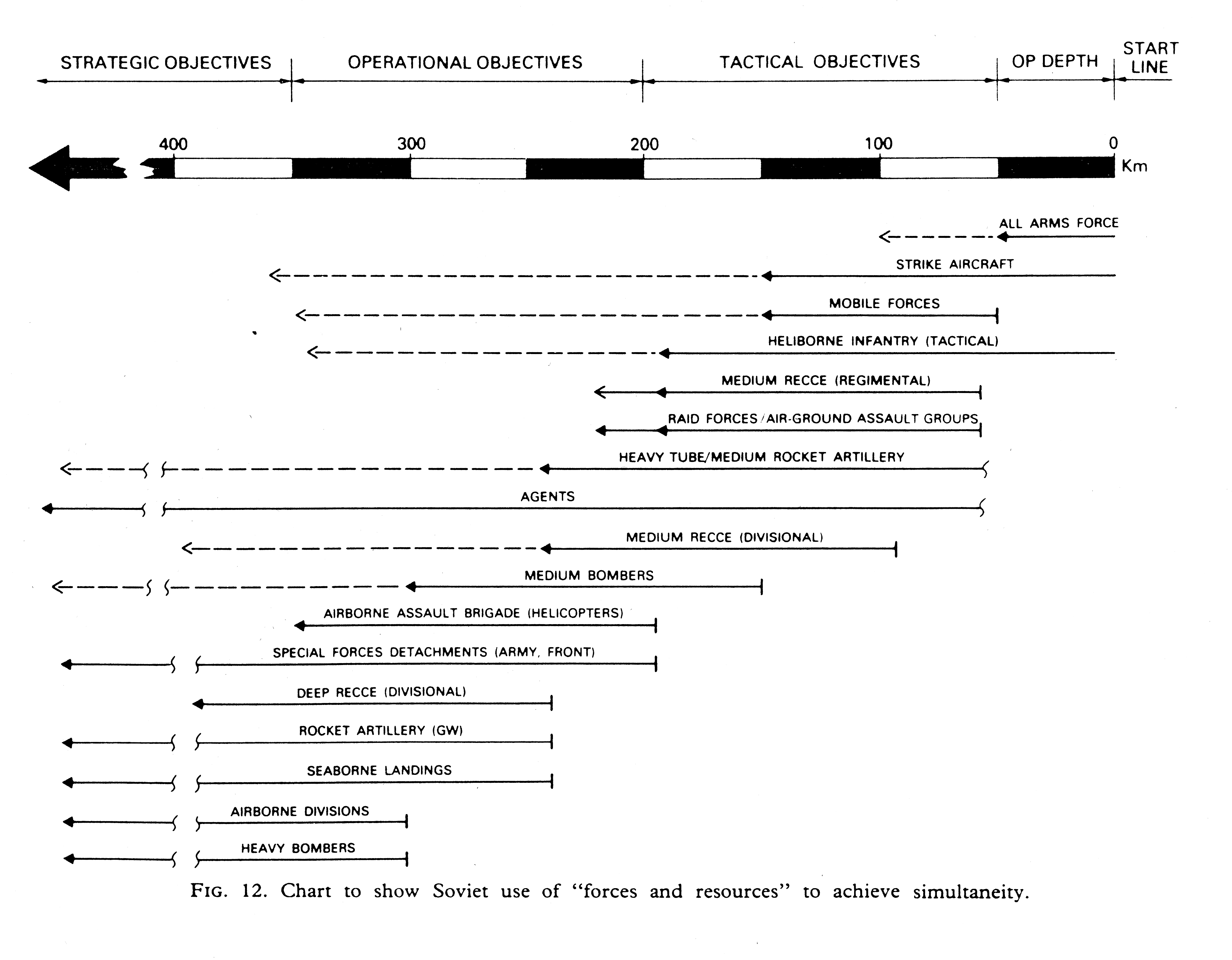
Briefly and in the most general terms possible, I suggest that the long-term effect of dominant firepower will be threefold. It will disperse mass in the form of a “net” of small detachments with the dual role of calling down fire and of local quasi-guerrilla action. Because of its low density, the elements of this net will be everywhere and will thus need only the mobility of the boot. It will transfer mass, structurally from the combat arms to the artillery, and in deployment from the direct fire zone (as we now understand it) to the formation and protection of mobile fire bases capable of movement at heavy-track tempo (Chapter 9). Thus the third effect will be to polarise mobility, for the manoeuvre force still required is likely to be based on the rotor. This line of thought is borne out by recent trends in Soviet thinking on the offensive. The concept of an operational manoeuvre group (OMG) which hives off raid forces against C3 and indirect fire resources is giving way to more fluid and discontinuous manoeuvre by task forces (“air-ground assault groups” found by “shock divisions”) directed onto fire bases—again of course with an operational helicopter force superimposed. [Simpkin, Race To The Swift, p. 169]
It seems to me that in the mid-1980s, Simpkin accurately predicted the emergence of modern anti-access/area denial (A2/AD) defensive systems with reasonable accuracy, as well the evolving thinking on the part of the U.S. military as to how to operate against them.
Simpkin’s vision of task forces (more closely resembling Russian/Soviet OMGs than rotary wing “air-ground assault groups” operational forces, however) employing “fluid and discontinuous manoeuvre” at operational depths to attack long-range precision firebases appears similar to emerging Army thinking about future multidomain operations. (It’s likely that Douglas MacGregor’s Reconnaissance Strike Group concept more closely fits that bill.)
One thing he missed on was his belief that rotary wing helicopter combat forces would supplant armored forces as the primary deep operations combat arm. However, there is the potential possibility that drone swarms might conceivably take the place in Simpkin’s operational construct that he allotted to heliborne forces. Drones have two primary advantages over manned helicopters: they are far cheaper and they are far less vulnerable to enemy fires. With their unique capacity to blend mass and fires, drones could conceivably form the deep strike operational hammer that Simpkin saw rotary wing forces providing.
Just as interesting was Simpkin’s anticipation of the growing importance of information and electronic warfare in these environments. More on that later.
Richard Simpkin on 21st Century Trends in Mass and Firepower
For my money, one of the most underrated analysts and theorists of modern warfare was the late Brigadier Richard Simpkin. A retired British Army World War II veteran, Simpkin helped design the Chieftan tank in the 60s and 70s. He is best known for his series of books analyzing Soviet and Western military theory and doctrine. His magnum opus was Race To The Swift: Thoughts on Twenty-First Century Warfare, published in 1985. A brilliant blend of military history, insightful analysis of tactics and technology as well as operations and strategy, and Simpkin’s idiosyncratic wit, the observations in Race To The Swift are becoming more prescient by the year.
Some of Simpkin’s analysis has not aged well, such as the focus on the NATO/Soviet confrontation in Central Europe, and a bold prediction that rotary wing combat forces would eventually supplant tanks as the primary combat arm. However, it would be difficult to find a better historical review of the role of armored forces in modern warfare and how trends in technology, tactics, and doctrine are interacting with strategy, policy, and politics to change the character of warfare in the 21st Century.
To follow on my previous post on the interchangeability of fire (which I gleaned from Simpkin, of course), I offer this nugget on how increasing weapons lethality would affect 21st Century warfare, written from the perspective of the mid 1980s:
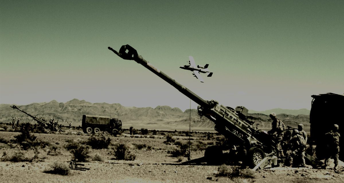
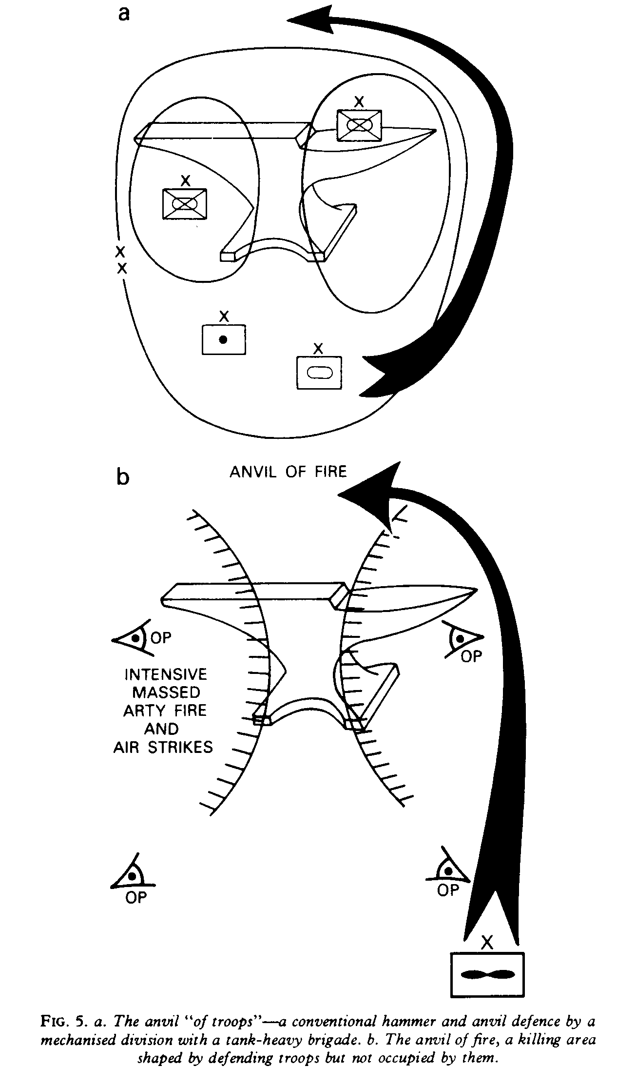
While accidents of ground will always provide some kind of cover, the effect of modern firepower on land force tactics is equally revolutionary. Just as we saw in Part 2 how the rotary wing may well turn force structures inside out, firepower is already turning tactical concepts inside out, by replacing the anvil of troops with an anvil of fire (Fig. 5, page 51)*. The use of combat troops at high density to hold ground or to seize it is already likely to prove highly costly, and may soon become wholly unprofitable. The interesting question is what effect the dominance of firepower will have at operational level.
One school of thought, to which many defence academics on both sides of the Atlantic subscribe, is that it will reduce mobility and bring about a return to positional warfare. The opposite view is that it will put a premium on elusiveness, increasing mobility and reducing mass. On analysis, both these opinions appear rather simplistic, mainly because they ignore the interchangeability of troops and fire…—in other words the equivalence or complementarity of the movement of troops and the massing of fire. They also underrate the part played by manned and unmanned surveillance, and by communication. Another factor, little understood by soldiers and widely ignored, is the weight of fire a modern fast jet in its strike configuration, flying a lo-lo-lo profile, can put down very rapidly wherever required. With modern artillery and air support, a pair of eyes backed up by an unjammable radio and perhaps a thermal imager becomes the equivalent of at least a (company) combat team, perhaps a battle group. [Simpkin, Race To The Swift, pp. 168-169]
Sound familiar? I will return to Simpkin’s insights in future posts, but I suggest you all snatch up a copy of Race To The Swift for yourselves.
* See above.
Interchangeability Of Fire And Multi-Domain Operations
With the emergence of the importance of cross-domain fires in the U.S. effort to craft a joint doctrine for multi-domain operations, there is an old military concept to which developers should give greater consideration: interchangeability of fire.
This is an idea that British theorist Richard Simpkin traced back to 19th century Russian military thinking, which referred to it then as the interchangeability of shell and bayonet. Put simply, it was the view that artillery fire and infantry shock had equivalent and complimentary effects against enemy troops and could be substituted for one another as circumstances dictated on the battlefield.
The concept evolved during the development of the Russian/Soviet operational concept of “deep battle” after World War I to encompass the interchangeability of fire and maneuver. In Soviet military thought, the battlefield effects of fires and the operational maneuver of ground forces were equivalent and complementary.
This principle continues to shape contemporary Russian military doctrine and practice, which is, in turn, influencing U.S. thinking about multi-domain operations. In fact, the idea is not new to Western military thinking at all. Maneuver warfare advocates adopted the concept in the 1980s, but it never found its way into official U.S. military doctrine.
An Idea Who’s Time Has Come. Again.
So why should the U.S. military doctrine developers take another look at interchangeability now? First, the increasing variety and ubiquity of long-range precision fire capabilities is forcing them to address the changing relationship between mass and fires on multi-domain battlefields. After spending a generation waging counterinsurgency and essentially outsourcing responsibility for operational fires to the U.S. Air Force and U.S. Navy, both the U.S. Army and U.S. Marine Corps are scrambling to come to grips with the way technology is changing the character of land operations. All of the services are at the very beginning of assessing the impact of drone swarms—which are themselves interchangeable blends of mass and fires—on combat.
Second, the rapid acceptance and adoption of the idea of cross-domain fires has carried along with it an implicit acceptance of the interchangeability of the effects of kinetic and non-kinetic (i.e. information, electronic, and cyber) fires. This alone is already forcing U.S. joint military thinking to integrate effects into planning and decision-making.
The key component of interchangability is effects. Inherent in it is acceptance of the idea that combat forces have effects on the battlefield that go beyond mere physical lethality, i.e. the impact of fire or shock on a target. U.S. Army doctrine recognizes three effects of fires: destruction, neutralization, and suppression. Russian and maneuver warfare theorists hold that these same effects can be achieved through the effects of operational maneuver. The notion of interchangeability offers a very useful way of thinking about how to effectively integrate the lethality of mass and fires on future battlefields.
But Wait, Isn’t Effects Is A Four-Letter Word?
There is a big impediment to incorporating interchangeability into U.S. military thinking, however, and that is the decidedly ambivalent attitude of the U.S. land warfare services toward thinking about non-tangible effects in warfare.
As I have pointed out before, the U.S. Army (at least) has no effective way of assessing the effects of fires on combat, cross-domain or otherwise, because it has no real doctrinal methodology for calculating combat power on the battlefield. Army doctrine conceives of combat power almost exclusively in terms of capabilities and functions, not effects. In Army thinking, a combat multiplier is increased lethality in the form of additional weapons systems or combat units, not the intangible effects of operational or moral (human) factors on combat. For example, suppression may be a long-standing element in doctrine, but the Army still does not really have a clear idea of what causes it or what battlefield effects it really has.
In the wake of the 1990-91 Gulf War and the ensuing “Revolution in Military Affairs,” the U.S. Air Force led the way forward in thinking about the effects of lethality on the battlefield and how it should be leveraged to achieve strategic ends. It was the motivating service behind the development of a doctrine of “effects based operations” or EBO in the early 2000s.
However, in 2008, U.S. Joint Forces Command commander, U.S Marine General (and current Secretary of Defense) James Mattis ordered his command to no longer “use, sponsor, or export” EBO or related concepts and terms, the underlying principles of which he deemed to be “fundamentally flawed.” This effectively eliminated EBO from joint planning and doctrine. While Joint Forces Command was disbanded in 2011 and EBO thinking remains part of Air Force doctrine, Mattis’s decree pretty clearly showed what the U.S. land warfare services think about battlefield effects.
Artillery Effectiveness vs. Armor (Part 5-Summary)
[This series of posts is adapted from the article “Artillery Effectiveness vs. Armor,” by Richard C. Anderson, Jr., originally published in the June 1997 edition of the International TNDM Newsletter.]
Posts in the series
Artillery Effectiveness vs. Armor (Part 1)
Artillery Effectiveness vs. Armor (Part 2-Kursk)
Artillery Effectiveness vs. Armor (Part 3-Normandy)
Artillery Effectiveness vs. Armor (Part 4-Ardennes)
Artillery Effectiveness vs. Armor (Part 5-Summary)
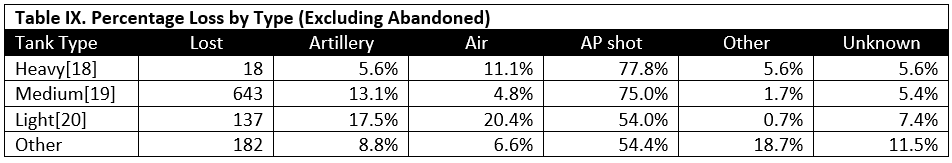
Table IX shows the distribution of cause of loss by type or armor vehicle. From the distribution it might be inferred that better protected armored vehicles may be less vulnerable to artillery attack. Nevertheless, the heavily armored vehicles still suffered a minimum loss of 5.6 percent due to artillery. Unfortunately the sample size for heavy tanks was very small, 18 of 980 cases or only 1.8 percent of the total.
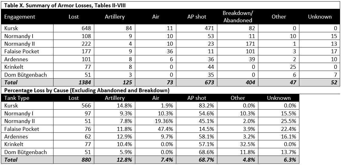 The data are limited at this time to the seven cases.[6] Further research is necessary to expand the data sample so as to permit proper statistical analysis of the effectiveness of artillery versus tanks.
NOTES
[18] Heavy armor includes the KV-1, KV-2, Tiger, and Tiger II.
[19] Medium armor includes the T-34, Grant, Panther, and Panzer IV.
[20] Light armor includes the T-60, T-70. Stuart, armored cars, and armored personnel carriers.
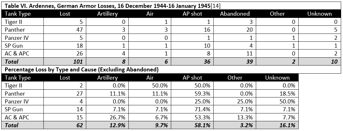
Artillery Effectiveness vs. Armor (Part 4-Ardennes)

[This series of posts is adapted from the article “Artillery Effectiveness vs. Armor,” by Richard C. Anderson, Jr., originally published in the June 1997 edition of the International TNDM Newsletter.]
Posts in the series
Artillery Effectiveness vs. Armor (Part 1)
Artillery Effectiveness vs. Armor (Part 2-Kursk)
Artillery Effectiveness vs. Armor (Part 3-Normandy)
Artillery Effectiveness vs. Armor (Part 4-Ardennes)
Artillery Effectiveness vs. Armor (Part 5-Summary)
 NOTES
NOTES
[14] From ORS Joint Report No. 1. A total of an estimated 300 German armor vehicles were found following the battle.
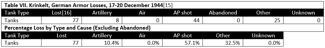
[15] Data from 38th Infantry After Action Report (including “Sketch showing enemy vehicles destroyed by 38th Inf Regt. and attached units 17-20 Dec. 1944″), from 12th SS PzD strength report dated 8 December 1944, and from strengths indicated on the OKW briefing maps for 17 December (1st [circa 0600 hours], 2d [circa 1200 hours], and 3d [circa 1800 hours] situation), 18 December (1st and 2d situation), 19 December (2d situation), 20 December (3d situation), and 21 December (2d and 3d situation).
[16] Losses include confirmed and probable losses.
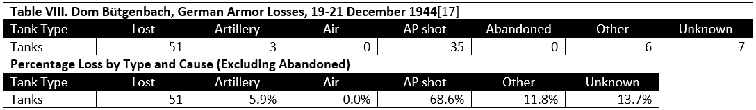
[17] Data from Combat Interview “26th Infantry Regiment at Dom Bütgenbach” and from 12th SS PzD, ibid.