Two conferences in Norway from 31 October to 2 November that might be of interest to people. They are both in Oslo in the same week, but at different hotels:
Was searching around on YouTube yesterday on “Dupuy Institute” and ran across this video: People Always Get This Wrong – YouTube. This was posted three weeks ago. Preston Stewart is not known to me.
I am called out by name on 5:14 in the video. It is clear he pulled up one of our old reports, the charts at 6:00 and 6:14 are ours. The chart at 6:36 is ours and was later republished in War by Numbers. It appears to be abbreviated. The complete chart is on page 10 of War by Numbers. The chart at 6:44 has also been republished in War by Numbers. The chart at 7:30 is from our reports. The one high odds attack that failed on that chart was an Iraqi attack against the coalition. See: TDI – The Dupuy Institute Publications.
Anyhow, would recommend that Mr. Stewart look at Trevor Dupuy’s Understanding War, Chapter 4: The Three-to-One Theory of Combat, and at my book War by Numbers, Chapter 2: Force Ratios.
Also, he might might the following blog posts are useful:
We do have a YouTube site: The Dupuy Institute – YouTube. So far the only video posted is a test video. The husky is named Max. We may be posting some more videos there in the next couple of months. There are three subscribers to our site. I gather we can get some funding if we get a 100,000 or more subscribers. So only 99,997 to go. Please subscribe.
A friend just pointed me to a recent 2019 paper done out at C&GSC at Leavenworth. It is called “An Examination of Force Ratios” and is by Major Joshua T. Christian. It is 37 pages. It is here: AD1083211.pdf (dtic.mil)
A few notes
“The nature of the inputs required for models such as the QJM or COFM mean that they are backwards looking, require numerous inputs, effort, and time to develop which limited their effectiveness to operational planners.”
3. Page 13: Hate to nit pick, but peak strength in Vietnam was higher and earlier than what he states. There are a number of other such statements in this paper I could argue with, but will avoid doing that. See Vietnam War chart drawn from page 274 of America’s Modern Wars: Insurgency & Counterinsurgency | Mystics & Statistics | Page 4 (dupuyinstitute.org).
5. Page 14: “This section highlights the work of operations research analysts, particularly those produced by the Historical Evaluation and Research Program (HERO), ad how it contributed to the Army’s transformation of the 1960s and 1970s.”
This is an odd statement. HERO was mostly historians. There were no OR people on staff, although people like Dr. Janice Fain, Robert McQuie and Dr. James Taylor were friends of Trevor Dupuy and provided independent inputs as friends and consultants. I was the first employee with some background in quantitative analysis of historical data (primarily from econometrics). It is part of the reason I was hired in 1987.
The idea that HERO “contributed to the Army’s transformation of the 1960s and 1970s” is jolting to me. All my experience is that in general, we tended to be ignored, downplayed or just dismissed. The Army’s support for what we do is clearly demonstrated by the low levels of funding that have been provided over the decades.
6. Page 15: “…establishing Dupuy as a prominent figure in the operational research field by the 1970s.”
7. Page 26: Now he gets to discussing me. I will try to withhold commenting too much.
8. Page 27: “Lawrence utilized the Tactical Numerical Deterministic Model (TNDM), which succeeded the QJM, to conduct his analysis, and more specifically to determine the winner and loser of an engagement, assess personnel and equipment losses, and determine the rate of advance.
No, I did not. I did not use the TNDM or any combat model for any of my analysis in the book. I did due a few simple statistical comparisons but did no combat modeling. He is not the first person to have made such mistake, which can only have come about by skimming my book (vice reading the whole thing) and then making false assumptions. I do have a chapter towards the end of the book that discuss some of the validation tests we ran using the TNDM, which is what seems to confuse people, but the TNDM was not used for any of the analysis in the book. He does correctly describe the validation tests of the model.
9. “As a result, the TNDM is more frequently used by companies to develop requirements that drive the development of hypothetical weapons more so than operation planners.”
10. Pages 31-32: In his discussion of insurgencies, it is clear has not seen my book America’s Modern Wars, or Dr. Andrew Hossack’s work or the work done by CAA on this using our databases (see pages 70-77 in America’s Modern Wars). He probably needs to.
There are 34 references to Dupuy in the paper, 11 references to The Dupuy Institute, 8 references to me (I know, very vain of me), 8 references to Dr. Janice Fain, 15 references to HERO, 17 references to the QJM and 15 references to the TNDM.
Units maneuver before and during a battle to achieve a more favorable position. This maneuver is often unopposed and is not the subject of this discussion. Unopposed movement before combat is often quite fast, although often not as fast as people would like to assume. Once engaged with an opposing force, the front line between them also moves, usually moving forwards if the attacker is winning and moving backwards for the defender if he is losing or choosing to withdraw. These are opposed advance rates. This section is focused on discussing opposed advance rates or “advance rates in combat.”
The operations research and combat modeling community have often taken a short-hand step of predicting advance rates in combat based upon force ratios, so that a force with a three-to-one force ratio advances faster than a force with a two-to-one force ratio. But, there is not a direct relationship between force ratios and advance rates. There is an indirect relationship between them, in that higher forces ratios increased the chances of winning, and winning the combat and the degree of victory helps increase advance rates. There is little analytical work that has been done on this subject.[1]
Opposed advance rates are very much influenced by 1) terrain, 2) weather and 3) the degree of mechanization and mobilization, in addition to 4) the degree of enemy opposition. These four factors all influence what the rates will be.
In a study The Dupuy Institute did on enemy prisoner of war capture rates, we ended up coding a series of engagements by outcome. This has proven to a useful coding for the examination of advance rates. Engagements codes as outcomes I and II (limited action and limited attack) are not of concern for this discussion. The engagement coded as attack fails (outcome III) is significant, as these are cases where the attacker is determined to have failed. As such they often do not advance at all, sometimes have a very limited advance and sometimes are even pushed back (have a negative advance). For example, in our work on the subject, of our 271 division-level engagements from Western Europe 1943-45 the average advance rate was 1.81 kilometers per day. For Eastern Europe in 1943 the average advance rate was 4.54 kilometers per day based upon 173 division-level engagements.[2] These advance rates are irrespective of what the force ratios are for an engagement.
In contrast, in those engagements where the attacker is determined to have won and is coded as attacker advances (outcome IV) the attacker advances an average of 2.00 kilometers in the 142 engagements from Western Europe 1943-45. The average force ratio of these engagements was 2.17. In the case of Eastern Europe in 1943, the average advance rate was 5.80 kilometers based upon 73 engagements. The average force ratio of these engagements was 1.62.
We also coded engagements where the defender was penetrated (outcome V). These are those cases where the attacker penetrated the main defensive line of the defending unit, forcing them to either withdraw, reposition or counterattack. This penetration is achieved by either overwhelming combat power, the end result of an extended operation that finally pushes through the defenses, or a gap in the defensive line usually as a result of a mistake. Superior mechanization or mobility for the attacker can also make a difference. In those engagements where the defender was determined to have been penetrated the attacker advanced an average of 4.12 kilometers in 34 engagements from Western Europe 1943-45. The average force ratio of these engagements was 2.31. In the case of Eastern Europe in 1943, the average advance rates was 11.28 kilometers based upon 19 engagements. The average force ratio of these engagements was 1.99.
This clearly shows the difference in advance rate based upon outcome. It is only related to force ratios to the extant the force ratios are related to producing these different outcomes.
Also of significance is terrain and weather. Needless to say, significant blocking obstacles like bodies of water, can halt an advance and various rivers and creeks often considerably slow them, even with engineering and bridging support. Rugged terrain is more difficult to advance through and easier to defend and delay then smoother terrain. Closed or wooded terrain is more difficult to advance through and easier to defend and delay then open terrain. Urban terrain tends to also slow down advance rates, being effectively “closed terrain.” If it is raining then advance rates are slower than in clear weather. Sometimes considerably slower in heavy rain. The season it is, which does influence the amount of daylight, also affects the advance rate. Units move faster in daylight than in darkness. This is all heavily influenced by the road network and the number of roads in the area of advance.
No systematic study of advance rates has been done by the operations research community. Probably the most developed discussion of the subject was the material assembled for the combat models developed by Trevor Dupuy. This included addressing the effects of terrain and weather and road network on the advance rates. A combat model is an imperfect theory of combat.
Even though this combat modeling effort is far from perfect and fundamentally based upon quantifying factors derived by professional judgment, tables derived from this modeling effort have become standard presentations in a couple of U.S. Army and USMC planning and reference manuals. This includes U.S. Army Staff Reference Guide and the Marine Corps’ MAGTF Planner’s Reference Manual.[3]
The original table, from Numbers, Predictions and War, is here:[4]
STANDARD (UNMODIFIED) ADVANCE RATES
Rates in km/day
Armored Mechzd. Infantry Horse Cavalry
Division Division Division Division or
or Force Force
Against Intense Resistance
(P/P: 1.0-1.1O)
Hasty defense/delay 4.0 4.0 4.0 3.0
Prepared defense 2.0 2.0 2.0 1.6
Fortified defense 1.0 1.0 1.0 0.6
Against Strong/Intense Resistance
(P/P: 1-11-125)
Hasty defense/delay 5.0 4.5 4.5 3.5
Prepared defense 2.25 2.25 2.25 1.5
Fortified defense 1.25 1.25 1.25 0.7
Against Strong Defense
(P/P: 1.26-1.45)
Hasty defense/delay 6.0 5.0 5.0 4.0
Prepared defense 2.5 2.5 2.5 2.0
Fortified defense 1.5 1.5 1.5 0.8
Against Moderate/Strong Resistance
(P/P: 1.46-1.75)
Hasty defense 9.0 7.5 6.5 6.0
Prepared defense 4.0 3.5 3.0 2.5
Fortified defense 2.0 2.0 1.75 0.9
Against Moderate Resistance
(P/P: 1.76-225)
Hasty defense/delay 12.0 10.0 8.0 8.0
Prepared defense 6.0 5.0 4.0 3.0
Fortified defense 3.0 2.5 2.0 1.0
Against Slight/Moderate Resistance
(P/P:2.26-3.0)
Hasty defense/delay 16.0 13.0 10.0 12.0
Prepared defense 8.0 7.0 5.0 6.0
Fortified defense 4.0 3.0 2.5 2.0
Against Slight Resistance
(P/P: 3.01-4.25)
Hasty defense/delay 20.0 16.0 12.0 15.0
Prepared defense 10.0 8.0 6.0 7.0
Fortified defense 5.0 4.0 3.0 4.0
Against Negligible/Slight Resistance
(P/P:4.26-6.00)
Hasty defense/delay 40.0 30.0 18.0 28.0
Prepared defense 20.0 16.0 10.0 14.0
Fortified defense 10.0 8.0 6.0 7.0
Against Negligible Resistance
(P/P: 6.00 plus)
Hasty defense /delay 60.0 48.0 24.0 40.0
Prepared/fortified defense 30.0 24.0 12.0 12.0
*Based on HERO studies: ORALFORE, Barrier Effectiveness, and Combat Data Subscription Service.
** For armored and mechanized infantry divisions, these rates can be sustained for 10 days only; for the next 20 days standard rates for armored and mechanized infantry forces cannot exceed half these rates.
This is a modeling construct built from historical data. These are “unmodified” rates. The modifications include: 1) General Terrain Factors (ranging from 0.4 to 1.05 for Infantry (combined arms) Force and from 0.2 to 1.0 for Cavalry or Armored Force, 2) Road Quality Factors (addressing Road Quality from 0.6 to 1.0 and Road Density from 0.6 to 1.0), 3) Obstacles Factors (ranging from 0.5 to 0.9 for both a River or steam and for Minefields), 4) Day/Night with night advance rate one-half of daytime advance rate and 5) Main Effort Factor (ranging from 1.0 to 1.2). These last five sets of tables are not shown here, but can be found in his writings.[5]
[1] The most significant works we are aware of is Trevor Dupuy’s ORALFORE study in 1972: Opposed Rates of Advance in Large Forces in Europe (ORALFORE), (TNDA, for DCSOPS, 1972); Trevor Dupuy’s 1979 book Numbers, Predictions and War; and a series of three papers by Robert Helmbold (Center for Army Analysis): “Rates of Advance in Land Combat Operations, June 1990,” “Survey of Past Work on Rates of Advance, and “A Compilation of Data on Rates of Advance.”
[2] See paper on the subject by Christopher A. Lawrence, “Advance Rates in Combat based upon Outcome,” posted on the blog Mystics & Statistic, April 2023. In the databases, there were 282 Western Europe engagements from September 1943 to January 1945. There were 256 Eastern Front engagements from February, March, July and August of 1943.
[3] See U.S. Army Staff Reference Guide, Volume I: Unclassified Resources, December 2020, ATP 5-0.2-1, pages xi and 220; and MAGTF Planner’s Reference Manual, MSTF pamphlet 5-0.3, October 2010, page 79. Both manuals include a table for division-level advances which is derived from Trevor Dupuy’s work, and both manuals contain a table for brigade-level and below advances which are calculated per hour that appear to also be derived from Trevor Dupuy’s division-level table. The U.S. Army manual gives the “brigade and below” advance rates in km/hr while the USMC manual, which appears to be the same table, gives the “brigade and below” advance rates in km/day. This appears to be a typo.
[4]Numbers, Predictions and War, pages 213-214. The sixth line of numbers, three numbers were changes from 1.85 to 1.25 as this was obviously a typo in the original.
[5] See Numbers, Predictions and War, pages 214-216.
What catches my attention about this article is the discussion of whether “troop-to-task” ratios, also known as tie-down ratios, sometimes also known as force ratios; should be measured based upon population or based upon insurgent strength.
To quote from his article: “Throughout the Iraq and Afghanistan campaigns, American analysts and military officials referred to a 20:1,000 (2%) troop-to-population ratio for successful counterinsurgency.”
He also notes: “These troop-to-population security ratios are notoriously unreliable and have weak empirical basis for planning.”
That is more polite than how I refer to them in private. I did discuss this subject on pages 70-71 of my book America’s Modern Wars.
He then states: “Another popular way to analyze troop requirements in through troop–to-insurgent ratios.”
Popular? I have not seen anyone do this in recent times. I do have a book published on the subject (America’s Modern Wars). Perhaps I am missing out on something that is going on in the basement of the Pentagon.
He does note that “This approach falls apart at step one: Counting insurgents.”
I have a chapter on the subject (Chapter 11: Estimating Insurgent Force Size, pages 115-120). It is possible. It is not perfect or easy; but doing something vague and difficult is better than doing something that is conceptually flawed. To date, I have not seen anyone else do anything further on estimating insurgents. My work was a tentative first cut on the subject. My customers were completely uninterested in this analysis, and nothing further was done. Clearly something further needs to be done. I think that is better than doing something that is conceptually flawed.
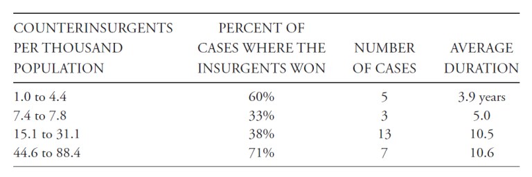
I have discussed this before on this blog and in my book: America’s Modern Wars. My discussion of the previous RAND work on the subject is on pages 70-71. It includes the following table from our work:
If anyone can tell me from that table where a 2% figure could come from, have at it.
Listed below are a collection of four relevant blog posts on the subject (there are some 1,288 posts on this blog). We do have categories like “Insurgency and Counterinsurgency,” “Force Ratios” and “Estimating Insurgent Force Size” this blog. We have done a few posts on the subject.
Needless to say, I think that basing the “troop-to-task” ratios on population is at best marginally relevant. For example, the troop-to-task ratio for Vietnam was 88.4. We did not win that one. On the other hand, when the Symbionese Liberation Army (SLA) with its two dozen members, raised hell in San Francisco and Los Angeles in the early 1970s, doing a political assassination, kidnapping Patty Hearst, and robbing banks, we took care of it using the LA police. We did not need to deploy 2% of the population of the United States (estimated at 213 million in 1974) to deal with the SLA. We did not need to raise over 4 million troops to suppress this insurgency.
I do think the size of the insurgency is relevant.
The last two posts I made on force ratios was drawn from my book War by Numbers. There are additional posts I did early last year on the subject based upon my in-process follow-on book More War by Numbers. They are summarized here:
I have been fairly diligent about making sure the “categories” that are listed on the right hand column of the blog are maintained. Therefore, clicking on Force Ratio will lead you to all 29 Force Ratio related posts on this blog. There are 1,129 posts on this blog (as of this post).
Now, the purpose of War by Numbers was not to create Combat Results Tables (CRT) for wargames. Its real purpose was to test the theoretical ideas of Clausewitz, and more particularly, Trevor N. Dupuy to actual real-world data. Not as case studies, but as statistical compilations that would show what the norms are. Unfortunately, military history is often the study of exceptions, or exceptional events, and what is often lost to the casual reader it what the norms are. Properly developed statistical database will clearly show what the norms are and how frequent or infrequent these exceptions are. People tend to remember the exceptional cases, they tend to forget the norms, if they even knew what they were to start with.
Chapters 3, 4 and 5 of War by Numbers is primarily focused on measuring human factors (which some people in the U.S. DOD analytical community seem to think are unmeasurable, even though we are measuring them). As part of that effort I ended up assemble a set of force ratios tables based upon theater and nationality. The first of these, on page 10, was in my previous blog post. Here are a few others, from page 11 of War by Numbers.
Germans attacking Soviets (Battles of Kharkov and Kursk), 1943
Force Ratio Result Percent Failure Number of cases
0.63 to 1.06-to-1.00 Attack usually succeeds 20% 5
1.18 to 1.87-to-1.00 Attack usually succeeds 6% 17
1.91-to-1.00 and higher Attacker Advances 0% 21
Soviets attacking Germans (Battles of Kharkov and Kursk), 1943
Force Ratio Result Percent Failure Number of cases
0.40 to 1.05-to-1 Attack usually fails 70% 10
1.20 to 1.65-to-1.00 Attack often fails 50% 11
1.91 to 2.89-to-1.00 Attack sometimes fails 44% 9
Pacific Theater of Operations (PTO) Data, U.S. attacking Japanese, 1945
Force Ratio Result Percent Failure Number of cases
1.40 to 2.89-to-1.00 Attack succeeds 0% 20
2.92 to 3.89-to-1.00 Attack usually succeeds 21% 14
4.35-to-1.00 and higher Attack usually succeeds 4% 26
Page 10 for War by Numbers includes the following table:
European Theater of Operations (ETO) Data, 1944
Force Ratio Result Percent Failure Number of cases
0.55 to 1.01-to-1.00 Attack Fails 100% 5
1.15 to 1.88-to-1.00 Attack usually succeeds 21% 48
1.95 to 2.56-to-1.00 Attack usually succeeds 10% 21
2.71-to-1.00 and higher Attacker Advances 0% 42
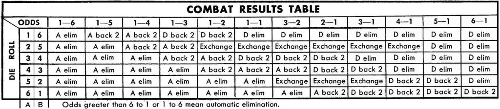
Many commercial wargames have something called a CRT or Combat Results Table. It is based upon force ratios. For example, this was one of the earliest CRTs used on Avalon Hill Games in the 1960s.
As can been seen from this Combat Results Table, at 1-to-1 the chances of an attack winning is one-in-three. At 2-to-1 odds the chances of the attacker winning is either the same as the defender winning or is a two-thirds chance of winning. At 3-to-1 odds, the attacker will always win.
Now the variable factor is the exchange result, which is defined that the defender removed everyone and the attacker removes as much as the defender. This usually results in an attacker win, if the attack has the right “spare change.” If the attacker was attacking with a single 7 strength unit against a 3 strength defender and they roll and exchange, then both units are eliminated.
Compare that to the table from my book based upon 116 division-level engagements from the European Theater of Operations (1944-145).
Needless to say, some elements of my book War by Numbers are of interest to the commercial wargaming community.
As a result of a comment by Tom from Cornwall, we ended up adding three posts to this discussion that looked at terrain and amphibious operations and river crossings in Italy:
The previous posts on this discussion on force ratios are presented here. These were the posts examining the erroneous interpretation of the three-to-one rule as presented in Army FM 6-0 and other publications:
We are going to end this discussion for now. There is some additional data from the European Theater of Operations (ETO) and Ardennes that we have assembled, but it presents a confusing picture. This is discussed in depth in War by Numbers (pages 32-48).
I am assembling these discussions on force ratios and terrain into the opening chapters for a follow-on book to War by Numbers.
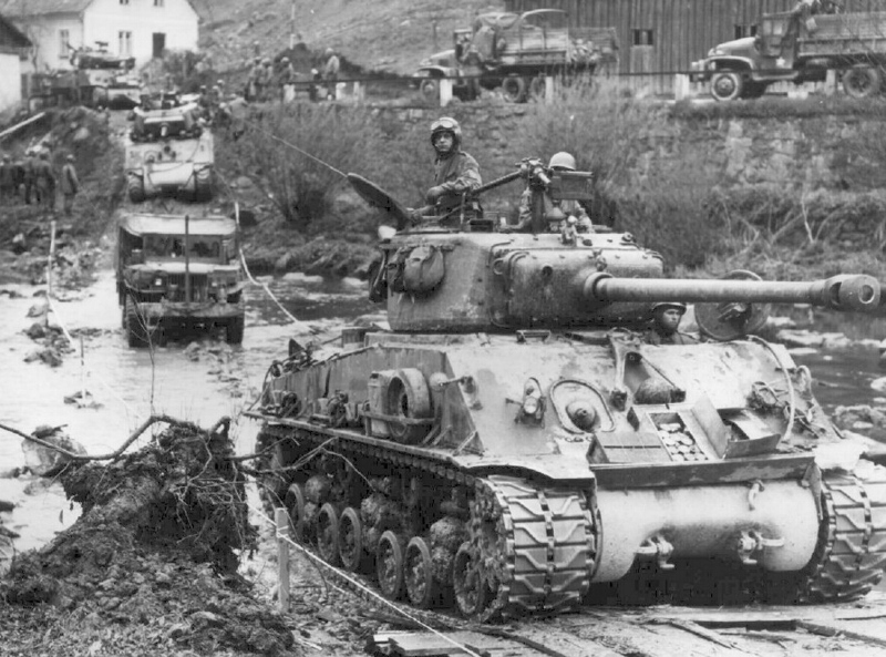
Polish Sherman III after battle on Gothic Line, Italy, September 1944
Having looked at casualty exchanges from my book War by Numbers and in the previous post, it is clear that there are notable differences between the German and Soviet armies, and between the Israeli and Arab armies. These differences show up in the force ratio tables, in the percent of wins, and in the casualty exchange ratios. As shown above, there is also a difference between the German and the U.S. and UK armies in Italy 1943-44, but this difference is no where to the same degree. These differences show up in the casualty exchange ratios. They also will show up in the force ratio comparisons that follow.
The Italian Campaign is an untapped goldmine for research into human factors. In addition to German, American and British armies, there were Brazilian, Canadian, French, French Algerian, French Moroccan, Greek, Indian, Italian, New Zealander, Polish, and South African forces there, among others like the Jewish brigade. There was also an African-American Division and a Japanese-American battalion and regiment actively engaged in this theater. Also the German records are much better than they were in the second half of 1944. So, the primary source data these engagements are built from are better than the engagements from the ETO.
We have 137 engagements from the Italian Campaign. There are 136 from 9 September to 4 June 1944 and one from13-17 September 1944. Of those, 70 consisted of the Americans attacking, 49 consisted of armed forces of the United Kingdom in the offense, and 18 consisted of the Germans attacks, often limited and local counterattacks (eight attacks against the United States and ten attacks against the UK). So, let us compare these based upon force ratios.
American Army attacking the German Army, Italy 1943-44
(70 cases in the complete data set, 62 cases in the culled data set)
Force Ratio……………Percent Attacker Wins………………..Number of Cases
There were seven cases of engagements coded as “limited attacks” and one case of “other”. These eight cases are excluded in the table above on those lines in italics.
Needless to say, this is a fairly good performance by the American Army, with them winning more than 40% the attacks below two-to-one and pretty winning most of them (86%) at odds above two-to-one.
British Army attacking the German Army, Italy 1943-44
(49 cases in the complete data set, 39 cases in the culled data set)
Force Ratio………………..Percent Attacker Wins………………..Number of Cases
There were five cases of limited action and five cases of limited attack. These ten cases are excluded in the table above on those lines in italics.
This again shows the difference in performance between the American Army and the British Army. This is always an uncomfortable comparison, as this author is somewhat of an anglophile with a grandfather from Liverpool; but data is data. In this case they won 44% of the time at attacks below two-to-one, which is similar to what the U.S. Army did. But then, they only won only 63% of the time at odds above two-to-one (using the culled data set). This could just be statistical anomaly as we are only looking at 30 cases, but is does support the results we are seeing from the casualty data.
What is interesting is the mix of attacks. For the American Army 77% of the attacks were at odds below two-to-one, for the British Army only 23% of the attacks were at odds below two-to-one (using the culled data sets). While these 99 cases do not include every engagement in the Italian Campaign at that time, they include many of the major and significant ones. They are probably a good representation. This does probably reflect a little reality here, in that the British tended to be more conservative on the attack then the Americans. This is also demonstrated by the British lower average loss per engagement.[7]
The reverse, which is when the Germans are attacking, does not provide a clear picture.
German Army attacking the American and British Army, Italy 1943-44 – complete data set (18 cases)
Force Ratio…………………..Percent Attacker Wins…………………Number of Cases
0.72 to 0.84………………………….0%………………………………………………7
1.17 to 1.48………………………..50…………………………………………………6
1.89…………………………………….0…………………………………………………1
2.16 to 2.20………………………..50…………………………………………………2
Gap in data
3.12 to 3.24………………………..50…………………………………………………2
The Germans only win in 28% of the cases here. They win in 13% of the engagements versus the U.S. (8 cases) and 40% of the engagements the UK (10 cases). Still, at low odds attacks (1.17 to 1.48-to-1) they are winning 50% of the time. They are conducting 78% of their attacks at odds below two-to-one.
In the end, the analysis here is limited by the number of cases. It is hard to draw any definitive conclusions from only 18 cases of attacks. Clearly the analysis would benefit with a more exhaustive collection of engagements from the Italian Campaign. This would require a significant investment of time (and money).[8]
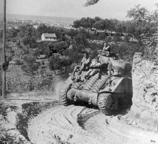
Regiment de Trois-Rivieres tanks entering the ruins of Regabuto, August 4th, 1943. Source: http://www.sfu.ca/tracesofthepast/wwii_html/it.htm
————————–
[1] There were four limited attacks that resulted in three defender wins and a draw. There was one “other” that was an attacker win.
[2] There three limited attacks that resulted in two defender wins and a draw.
[3] There were four “limited actions” that were defender wins and one “limited attack” that was a defender win.
[4] There as one “limited action” that was a defender win and two “limited attacks” that were defender wins.
[5] There were two “limited attacks” that were defender wins.
[6] The author’s grandfather was born in Liverpool and raised in Liverpool, England and Ryls, Wales. He served in the British merchant marine during World War I and afterwards was part of the British intervention at Murmansk Russia in 1918-1919. See the blog post:
[7] See War by Numbers, pages 25-27. The data shows that for the Americans in those 36 cases where their attack was successful they suffered an average of 353 casualties per engagement. For the 34 American attacks that were not successful they suffered an average of 351 casualties per engagement. For the UK, in the 23 cases where their attack was successful, the UK suffered an average of 213 casualties per engagement. Of the 26 cases where the UK attacks were not successful, they suffered an average of 137 casualties per engagement.
[8] Curt Johnson, the vice-president of HERO, estimated that it took an average of three man-days to create an engagement. He was involved in developing the original database that included about half of the 137 Italian Campaign engagements. My estimation parameter, including the primary source research required to conduct this is more like six days. Regardless, this would mean that just to create this 137 case database took an estimated 411 to 822 man-days, or 1.6 to 3.3 man-years of effort. Therefore, to expand this data set to a more useful number of engagements is going to take several years of effort.