Validating A Combat Model (Part XII)

[The article below is reprinted from April 1997 edition of The International TNDM Newsletter.]

The Second Test of the TNDM Battalion-Level Validations: Predicting Casualties
by Christopher A. Lawrence

FANATICISM AND CASUALTY INSENSITIVE SYSTEMS:

It was quite clear from looking at the battalion-level data before we did the validation runs that there appeared to be two very different loss patterns, based upon—dare I say it—nationality. See the article in issue 4 of the TNDM Newsletter, “Looking at Casualties Based Upon Nationality Using the BLODB.” While this is clearly the case with the Japanese in WWII, it does appear that other countries were also operating in a manner that produced similar casualty results. So, instead of using the word fanaticism, let’s refer to them as “casualty insensitive” systems. For those who really need a definition before going forward:

“Casualty Insensitive” System: A social or military system that places a high priority on achieving the objective or fulfilling the mission and o low priority on minimizing casualties. Such systems lend to be “mission obsessive” versus using some form of “cost benefit” method of weighing whether the objective is worth the losses suffered to take it.

EXAMPLES OF CASUALTY INSENSITIVE SYSTEMS:

For the purpose of the database, casualty sensitive systems were defined as the Japanese and all highly motivated communist-led armies. These include:

• Japanese Army, WWII
• Viet Mihn
• Viet Cong
• North Vietnamese
• Indonesian

We have included the Indonesians in this list even though it was based upon only one example.

In the WWII and post-WWII period, one would expect that the following armies would also be “casualty insensitive”

• Soviet Army in WWII
• North Korean Army
• Communist Chinese Army in Korea
• Iranian “Pasdaran“

Data can certainly be found to test these candidates.

One could postulate that the WWI attrition multiplier of 4 that we used also incorporates the 2.5 “casualty insensitive” multiplier. This would imply that there was only a multiplier of 1.6 to account for other considerations, like adjusting to the impact of increased firepower on the battlefield. One could also postulate that certain nations, like Russia, have had “casualty insensitive” systems throughout their last 100 years of history. This could also be tested by looking of battles over time of Russians versus Germans compared to Germans versus British, U.S. or French. One could easily carry this analysis back to the Seven Years’ War. If this was the case, this would establish a clear cultural basis for the “casualty insensitive” multiplier, but to do so would require the TNDM to be validated for periods before 1900. This would all be useful analysis in the future, but is not currently budgeted for.

It was expected that the “casualty insensitive” multiplier of 2.5 derived from the Japanese data would be too high to apply directly to the armies. Much to our surprise, we found that this did not appear to be the case. This partially or wholly explained the under-prediction of the 15 of our 20 significantly under-predicted post-WWII engagements. Time would explain another one. And four were not explained.

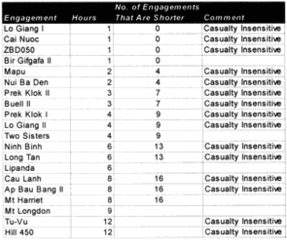
The model noticeably underestimated all the engagements under nine hours except Bir Gifgafa I (2 hours). Pearls AFB (4.5) and Wireless Ridge (8 hours). It noticeably under-estimated all the 15 “fanatic” engagements. If the formulations derived from the earlier data were used here (engagements less than 4 hours and fanatic), then there are 17 engagements in which one side is “casualty insensitive” or in which the engagement time is less than 4 hours. Using the above formulations then 17 engagements would have their casualty figures changed.

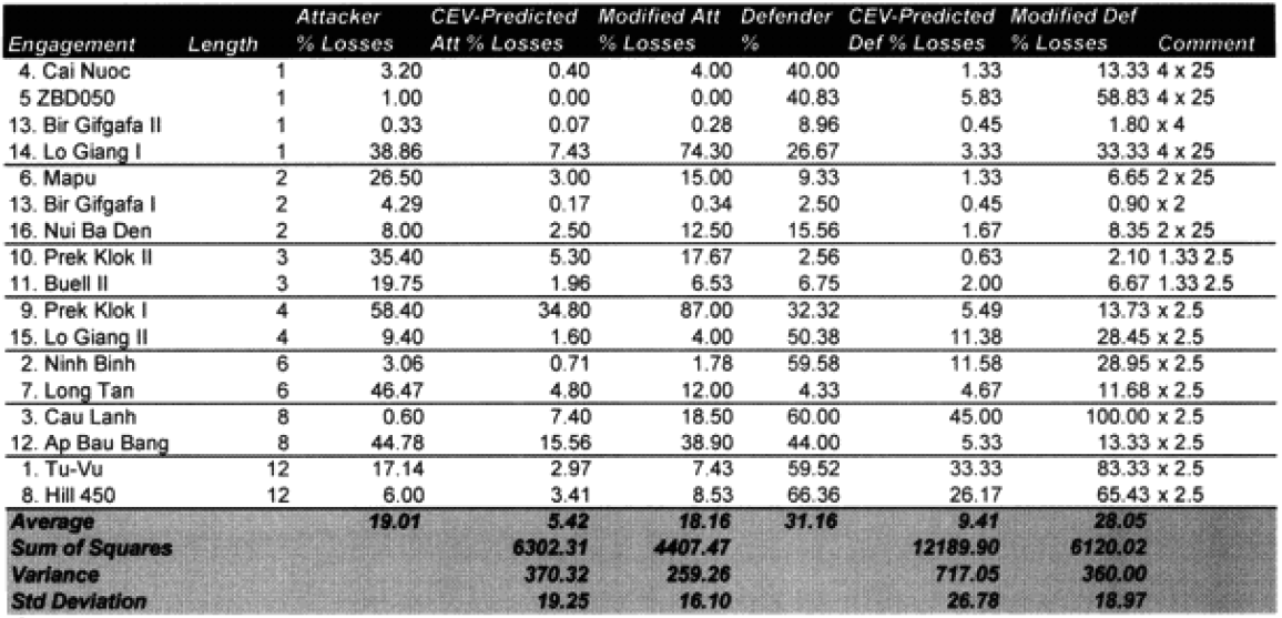
The modified percent loss figures are the CEV predicted percent loss times the factor for “casualty insensitive” systems (for those 15 cases where it applies) and times the formulation for battles less than 4 hours (for those 9 cases where it applies).

Looking at the table at the top of the next page, it would appear that we are on the correct path. But to be safe, on the next page let’s look at the predictive value of the 13 engagements for which we didn’t redefine the attrition multipliers.

The 13 engagements left unchanged:

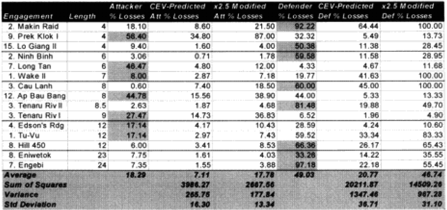
So, we are definitely heading in the right direction now. We have identified two model changes—time and “casualty insensitive.” We have developed preliminary formulations for time and for “casualty insensitive” forces. Unfortunately, the time formulation was based upon seven WWI engagements. The “casualty insensitive” formulation was based upon seven WWII engagements. Let’s use all our data in the first validation database here for the moment to come up with figures with which we can be more comfortable:

The highlighted entries in the table above indicate “casualty insensitive” forces. We are still struggling with the concept that having one side being casualty insensitive increases both sides’ losses equally. We highlighted them in an attempt to find any other patterns we were missing. We could not.

Now, there may be a more sophisticated measurement of this other than the brute force method of multiplying both sides by 2.5. This might include different multipliers depending on whether one is the fanatic vs non-fanatic side or different multipliers for attack or defense. First, I cannot find any clear indication that there should be a different multiplier for the attacker or defender. A general review of the data confirms that. Therefore, we are saying that the combat relationships between attacker and defender do not change in high intensity or casualty insensitive battles from those experienced in the norm.

What is also clear is that our multiplier of 2.5 appears to be about as good a fit as we can get from a straight multiplier. It does not appear that there is any significant difference between the attrition multiplier for types of “casualty insensitive” systems, whether they are done because of worship of the emperor or because the commissar will shoot slackers. Apparently the mode of fighting is more significant for measuring combat results than how one gets there, although certainly having everyone worship the emperor is probably easier to “administer.”

This still leaves us having to look at whether we should develop a better formulation for time.

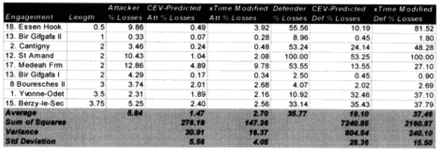
Non-fanatic engagement of less than 4 hours:

For fairly obvious reasons, we are still concerned about this formulation for battles of less than one hour, as we have only one example, but until we conduct the second validation, this formulation will remain as is.

Now the extreme cases:

List of all engagements less than 4 hours where one side was fanatic:

It would appear that these formulations of time and “casualty insensitivity” have passed their initial hypothesis formulations tests. We are now willing to make changes to the model based upon this and run the engagements from the second validation data base to test it.

Next: Predicting casualties: Conclusions