Validating A Combat Model (Part X)

[The article below is reprinted from April 1997 edition of The International TNDM Newsletter.]

The Second Test of the TNDM Battalion-Level Validations: Predicting Casualties
by Christopher A. Lawrence

TIME AND THE TNDM:

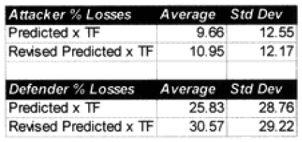
Before this validation was even begun, I knew we were going to have a problem with the fact that most of the engagements were well below 24 hours in length. This problem was discussed in depth in “Time and the TNDM,” in Volume l, Number 3 of this newsletter. The TNDM considers the casualties for an engagement of less than 24 hours to be reduced in direct proportion to that time. I postulated that the relationship was geometric and came up with a formulation that used the square root of that fraction (i.e. instead of 12 hours being .5 times casualties. it was now .75 times casualties). Being wedded to this idea, l tested this formulation in all ways and for several days, I really wasn’t getting a better fit. All I really did was multiply all the points so that the predicted average was closer. The top-level statistics were:

TF=Time Factor

I also looked out how the losses matched up by one of three periods (WWI, WWII. and post-WWII). When we used the time factor multiplier for the attackers, the WWI engagements average became too high, and the standard deviation increase, same with WWII, while the post-WWII averages were still too low, but the standard deviations got better. For the defender, we got pretty much the same pattern, except now the WWII battles were under-predicting, but the standard deviation was about the same. It was quite clear that all I had with this time factor was noise.

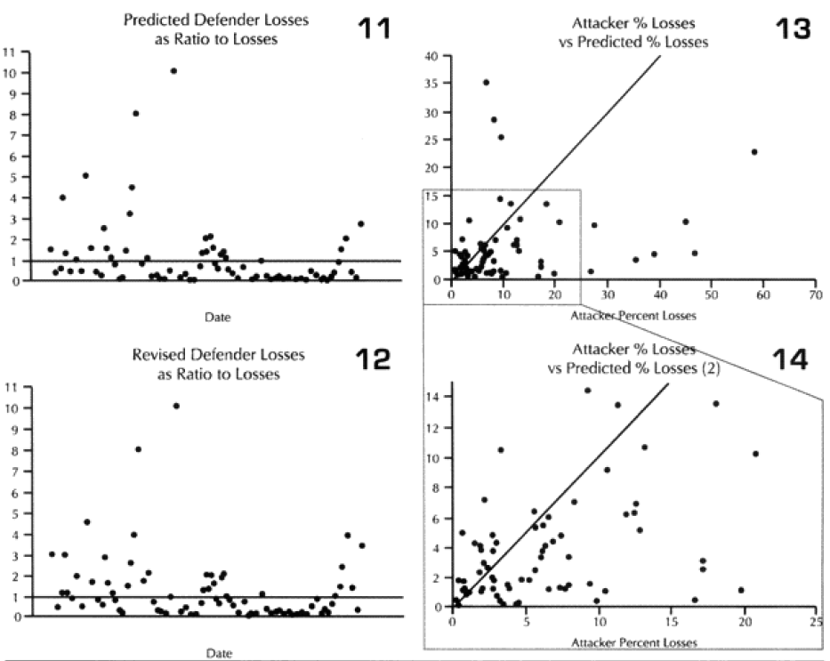
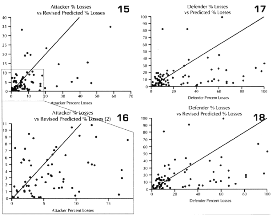Like any good chef, my failed experiment went right down the disposal. This formulation died a natural death. But looking by period where the model was doing well, and where it wasn’t doing well is pretty telling. The results were:

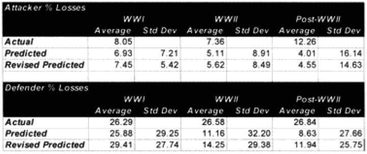Looking at the basic results. I could see that the model was doing just fine in predicting WWI battles, although its standard deviation for the defenders was still poor. It wasn’t doing very well with WWII, and performed quite poorly with modem engagements. This was the exact opposite effect to our test on predicting winners and losers, where the model did best with the post-WWII battles and worst with the WWI battles. Recall that we implemented an attrition multiplier of 4 for the WWI battles. So it was now time to look at each battle, and figure out where were we really off. In this case. I looked at casualty figures that were off by a significant order of magnitude. The reason l looked at significant orders of magnitude instead of percent error, is that making a mistake like predicting 2% instead of 1% is not a very big error, whereas predicting 20%, and having the actual casualties 10%, is pretty significant. Both would be off by 100%.

SO WHERE WERE WE REALLY OFF? (WWI)

In the case of the attackers, we were getting a result in the ball park in two-thirds of the cases, and only two cases—N Wood 1 and Chaudun—were really off. Unfortunately, for the defenders we were getting a reasonable result in only 40% of the cases, and the model had a tendency to under-or over-predict.

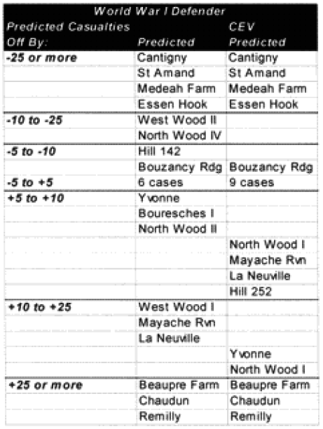It is clear that the model understands attacker losses better than defender losses. I suspect this is related to the model having no breakpoint methodology. Also, defender losses may be more variable. I was unable to find a satisfactory explanation for the variation. One thing I did notice was that all four battles that were significantly under-predicted on the defender sides were the four shortest WWI battles. Three of these were also noticeably under-predicted for the attacker. Therefore. I looked at all 23 WWI engagements related to time.

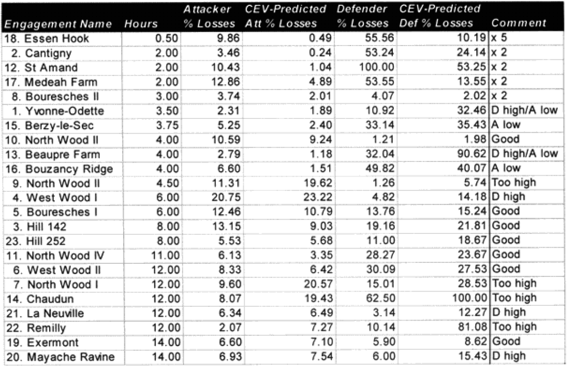Looking back at the issue of time, it became clear the model was clearly under-predicting in battles of less than four hours. I therefore came up with the following time scaling formula:

If time of battle less than four hours, then multiply attrition by (4/(Length of battle in hours)).

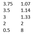What this formula does is make all battles less than four hours equal to a four-hour engagement. This intuitively looks wrong, but one must consider how we define a battle. A “battle” is defined by the analyst after the fact. The start time is usually determined by when the attack starts (or when the artillery bombardment starts) and end time by when the attack has clearly failed, or the mission has been accomplished, or the fighting has died down. Therefore, a battle is not defined by time, but by resolution.

As such, any battle that only lasts a short time will still have a resolution, and as a result of achieving that resolution there will be considerable combat experience. Therefore, a minimum casualty multiplier of 1/6 must be applied to account for that resolution. We shall see if this is really the case when we run the second validation using the new battles, which have a considerable number of brief engagements. For now, this seems to fit.

As for all the other missed predictions, including the over-predictions, l could not find a magic formula that connected them. My suspicion was that the multiplier of x4 would be a little too robust, but even after adjusting for the time equation, this left 14 of the attacker‘s losses under-predicted and six of the defender actions under-predicted. If the model is doing anything, it is under-predicting attacker casualties and over-predicting defender casualties. This would argue for a different multiplier for the attacker than for the defender (higher one for the attacker). We had six cases where the attacker‘s and defenders predictions were both low, nine where they were both high, and eight cases where the attackers prediction was low while the defender’s prediction was high. We had no cases where the attacker’s prediction was high and the defender’s prediction was low. As all these examples were from the western front in 1918, U.S. versus Germans, then the problem could also be that the model is under-predicting the effects of fortifications, or the terrain for the defense. It could also be indicative of a fundamental difference in the period that gave the attackers higher casualty rates than the defenders. This is an issue I would like to explore in more depth, and l may do so after l have more WWI data from the second validation.

Next: “Fanaticism” and casualties