
[The article below is reprinted from April 1997 edition of The International TNDM Newsletter.]
The Second Test of the TNDM Battalion-Level Validations: Predicting Casualties
by Christopher A. Lawrence
Actually, l was pretty pleased with the first test of the TNDM, predicting winners and losers. I wasn’t too pleased with how it did with WWI, but was quite pleased with its prediction of post-WWII combat. But l knew from our previous analysis that we were going to have some problems with the casualty prediction estimates for WWI, for any battles that the Japanese were involved with, and for shorter engagements.
The problems in prediction of casualties, as related to certain nationalities, were discussed in Trevor Dupuy’s Numbers, Predictions and War: Using History to Evaluate Combat Factors and Predict the Outcome of Battles (Indianapolis; New York: The Bobbs-Merrill Co., 1979). In the original QJM, as published in Numbers, Predictions, & War, three special conditions served as attrition multipliers. These were:
- For period 1900-1945. Russian and Japanese rates are double those calculated.
- For period 1914-1941, rates as calculated must be doubled; for Russian, Turkish, and Balkan forces they must be quadrupled.
- For 1950-1953 rate as calculated will apply for UN forces (other than ROK): for ROK. North Koreans, and Chinese rates are doubled.
The attrition calculation for the TNDM is different from that used in the QJM. Actually the attrition calculations for the later versions of the QJM differ from the earlier versions. The base casualty rates that are used in the original QJM are very different from those used in the TNDM. See my articles in the TNDM Newsletter, Volume 1, Issue 3. Basically the QJM starts with a based factor of 2.8% for attackers versus 4% for the TNDM, while its base factor for defenders is 1.5% versus 6% for the TNDM.
When Dave Bongard did the first TNDM runs for this validation effort, he automatically added in an attrition multiplier of 4 for all the WWI battles. This undocumented methodology was implemented by Mr. Bongard instinctively because he knew from experience that you need to multiply the attrition rates by 4 for WWI battles. I decided to let it stand and see how it measured up during the validation.
We then made our two model runs for each validation, first without the CEV, and a second run with the CEV incorporated. I believe the CEV results from this methodology are explained in the previous article on winners and losers.
At the top of the next column is a comparison of the attacker losses versus the losses predicted by the model (graphs 1 and 2). This is in two scales, so you can see the details of the data.
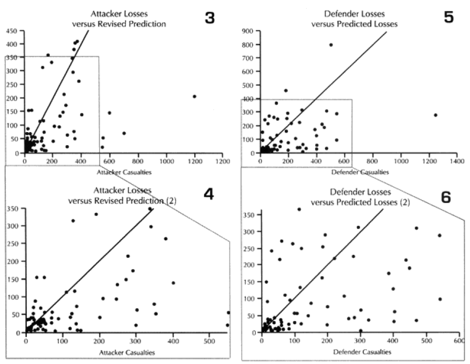
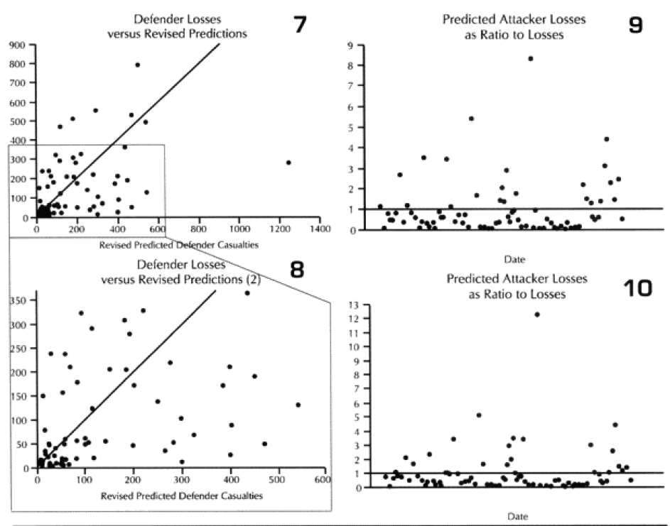
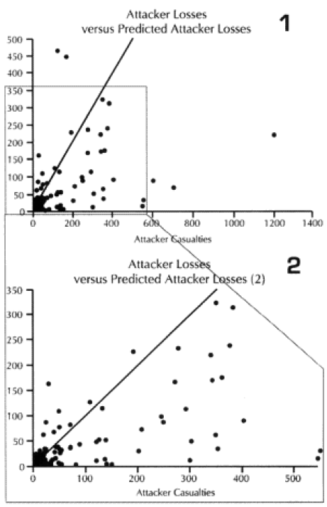 The diagonal line across these graphs and across the next seven graphs is the “perfect prediction” line, with any point on that line being perfectly predicted. The closer a point is to that line, the better the prediction. Points to the left of that line is where the model over-predicted casualties, while the points to the right is where the model under-predicted. We also ran the model using the CEV as predicted by the model. This “revised prediction” is shown in the next graph (see graphs 3 and 4). We also have done the same comparison of total casualties for the defender (see graphs 5 through 8).
 The model is clearly showing a tendency to under-predict. This is shown in the next set of graphs, where we divided the predicted casualties by the actual casualties. Values less than one are under-predictions. That means everything below the horizontal line shown on the graph (graph 9) is under-predicted. The same tests were done the “revised prediction“ (meaning with CEV) for the attacker and the both predictions for the defender (graphs 10-12).
I then attempted to do some work using the total casualty figures, followed by a series of meaningless tests of the data based upon force size. Force sizes range widely, and the size of forces committed to battle has a significant impact on the total losses. Therefore, to get anything useful, l really needed to look at percent of losses, not gross losses. These are displayed in the next 6 graphs (graphs 13-18).
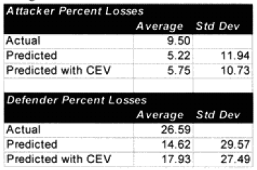
Comparing our two outputs (model prediction without CEV incorporated and model prediction with CEV incorporated) to the 76 historical engagements gives the following disappointing results:
 The standard deviation was measured by taking each predicted result, subtracting from it the actual result squaring it, summing all 76 cases, dividing by 76, and taking the square root. (see sidebar A Little Basic Statistics below.)
 First and foremost, the model was under-predicting by a factor of almost two. Furthermore it was running high standard deviations. This last result did not surprise me considering the nature of the battalion-level combat.
The addition of the CEVs did not significantly change the casualties. This is because in the attrition equations, the conditions of the battlefield play an important part in determining casualties. People in the past have claimed that the CEVs were some type of fudge factor. If that is the case, then it is a damned lousy fudge factor. If the TNDM is getting a good prediction on casualties, it is not because of a CEV “fudge factor.”
SIDEBAR: A Little Basic Statistics
The mean is 5.75 for the attacker and 17.93 for the defender, the standard deviation is 10.73 for the attacker and 27.49 for the defender. The number of examples is 76, the degree of freedom is 75. Therefore the confidence intervals are:
 With the actual average being 9.50, we are clearly predicting too low.
 With the actual average being 26.59, we are again clearly predicting too low.
Next: Time and casualty rates
