Validating A Combat Model (Part V)

[The article below is reprinted from April 1997 edition of The International TNDM Newsletter.]

The First Test of the TNDM Battalion-Level Validations: Predicting the Winners
by Christopher A. Lawrence

Part II

CONCLUSIONS:

WWI (12 cases):

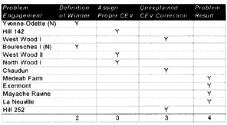
For the WWI battles, the nature of the prediction problems are summarized as:

CONCLUSION: In the case of the WWI runs, five of the problem engagements were due to confusion of defining a winner or a clear CEV existing for a side that should have been predictable. Seven out of the 23 runs have some problems, with three problems resolving themselves by assigning a CEV value to a side that may not have deserved it. One (Medeah Farm) was just off any way you look at it, and three suffered a problems because historically the defenders (Germans) suffered surprisingly low losses. Two had the battle outcome predicted correctly on the first run, and then had the outcome incorrectly predicted after a CEV was assigned.

With 5 to 7 clear failures (depending on how you count them), this leads one to conclude that the TNDM can be relied upon to predict the winner in a WWI battalion-level battle in about 70% of the cases.

WWII (8 cases):

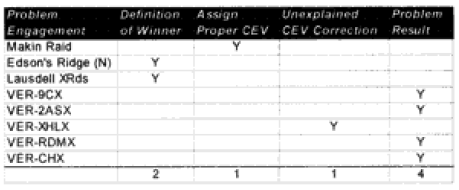
For the WWII battles, the nature of the prediction problems are summarized as:

CONCLUSION: In the case of the WWII runs, three of the problem engagements were due to confusion of defining a winner or a clear CEV existing for a side that should have been predictable. Four out of the 23 runs suffered a problem because historically the defenders (Germans) suffered surprisingly low losses and one case just simply assigned a possible unjustifiable CEV. This led to the battle outcome being predicted correctly on the first run, then incorrectly predicted after CEV was assigned.

With 3 to 5 clear failures, one can conclude that the TNDM can be relied upon to predict the winner in a WWII battalion-level battle in about 80% of the cases.

Modern (8 cases):

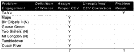
For the post-WWll battles, the nature of the prediction problems are summarized as:

CONCLUSION: ln the case of the modem runs, only one result was a problem. In the other seven cases, when the force with superior training is given a reasonable CEV (usually around 2), then the correct outcome is achieved. With only one clear failure, one can conclude that the TNDM can be relied upon to predict the winner in a modern battalion-level battle in over 90% of the cases.

FINAL CONCLUSIONS: In this article, the predictive ability of the model was examined only for its ability to predict the winner/loser. We did not look at the accuracy of the casualty predictions or the accuracy of the rates of advance. That will be done in the next two articles. Nonetheless, we could not help but notice some trends.

First and foremost, while the model was expected to be a reasonably good predictor of WWII combat, it did even better for modem combat. It was noticeably weaker for WWI combat. In the case of the WWI data, all attrition figures were multiplied by 4 ahead of time because we knew that there would be a fit problem otherwise.

This would strongly imply that there were more significant changes to warfare between 1918 and 1939 than between 1939 and 1989.

Secondly, the model is a pretty good predictor of winner and loser in WWII and modern cases. Overall, the model predicted the winner in 68% of the cases on the first run and in 84% of the cases in the run incorporating CEV. While its predictive powers were not perfect, there were 13 cases where it just wasn’t getting a good result (17%). Over half of these were from WWI, only one from the modern period.

In some of these battles it was pretty obvious who was going to win. Therefore, the model needed to do a step better than 50% to be even considered. Historically, in 51 out of 76 cases (67%). the larger side in the battle was the winner. One could predict the winner/loser with a reasonable degree of success by just looking at that rule. But the percentage of the time the larger side won varied widely with the period. In WWI the larger side won 74% of the time. In WWII it was 87%. In the modern period it was a counter-intuitive 47% of the time, yet the model was best at selecting the winner in the modern period.

The model’s ability to predict WWI battles is still questionable. It obviously does a pretty good job with WWII battles and appears to be doing an excellent job in the modern period. We suspect that the difference in prediction rates between WWII and the modern period is caused by the selection of battles, not by any inherit ability of the model.

RECOMMENDED CHANGES: While it is too early to settle upon a model improvement program, just looking at the problems of winning and losing, and the ancillary data to that, leads me to three corrections:

1. Adjust for times of less than 24 hours. Create a formula so that battles of six hours in length are not 1/4 the casualties of a 24-hour battle, but something greater than that (possibly the square root of time). This adjustment should affect both casualties and advance rates.
2. Adjust advance rates for smaller unit: to account for the fact that smaller units move faster than larger units.
3. Adjust for fanaticism to account for those armies that continue to fight after most people would have accepted the result, driving up casualties for both sides.

Next Part III: Case Studies