The Effects Of Dispersion On Combat

[The article below is reprinted from the December 1996 edition of The International TNDM Newsletter. A revised version appears in Christopher A. Lawrence, War by Numbers: Understanding Conventional Combat (Potomac Books, 2017), Chapter 13.]

The Effects of Dispersion on Combat
by Christopher A. Lawrence

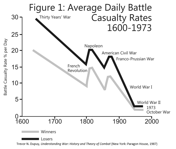
The TNDM[1] does not play dispersion. But it is clear that dispersion has continued to increase over time, and this must have some effect on combat. This effect was identified by Trevor N. Dupuy in his various writings, starting with the Evolution of Weapons and Warfare. His graph in Understanding War of the battle casualties trends over time is presented here as Figure 1. As dispersion changes over time (dramatically), one would expect the casualties would change over time. I therefore went back to the Land Warfare Database (the 605 engagement version[2]) and proceeded to look at casualties over time and dispersion from every angle that l could.

l eventually realized that l was going to need some better definition of the time periods l was measuring to, as measuring by years scattered the data, measuring by century assembled the data in too gross a manner, and measuring by war left a confusing picture due to the number of small wars with only two or three battles in them in the Land Warfare Database. I eventually defined the wars into 14 categories, so I could fit them onto one readable graph:

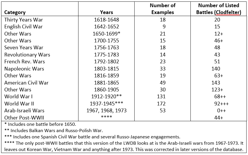To give some idea of how representative the battles listed in the LWDB were for covering the period, I have included a count of the number of battles listed in Michael Clodfelter’s two-volume book Warfare and Armed Conflict, 1618-1991. In the case of WWI, WWII and later, battles tend to be defined as a divisional-level engagement, and there were literally tens of thousands of those.

I then tested my data again looking at the 14 wars that I defined:

• Average Strength by War (Figure 2)
• Average Losses by War (Figure 3)
• Percent Losses Per Day By War (Figure 4)a
• Average People Per Kilometer By War (Figure 5)
• Losses per Kilometer of Front by War (Figure 6)
• Strength and Losses Per Kilometer of Front By War (Figure 7)
• Ratio of Strength and Losses per Kilometer of Front by War (Figure 8)
• Ratio of Strength and Loses per Kilometer of Front by Century (Figure 9)

A review of average strengths over time by century and by war showed no surprises (see Figure 2). Up through around 1900, battles were easy to define: they were one- to three-day affairs between clearly defined forces at a locale. The forces had a clear left flank and right flank that was not bounded by other friendly forces. After 1900 (and in a few cases before), warfare was fought on continuous fronts

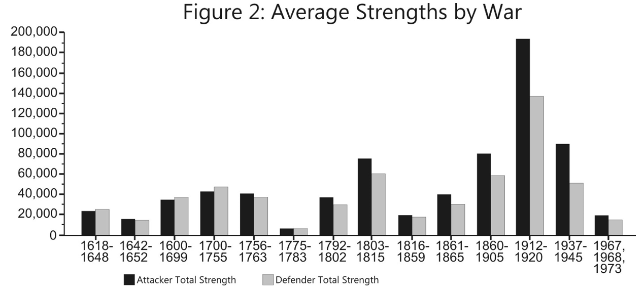with a ‘battle’ often being a large multi-corps operation. It is no longer clearly understood what is meant by a battle, as the forces, area covered, and duration can vary widely. For the LWDB, each battle was defined as the analyst wished. ln the case of WWI, there are a lot of very large battles which drive the average battle size up. ln the cases of the WWII, there are a lot of division-level battles, which bring the average down. In the case of the Arab-Israeli Wars, there are nothing but division and brigade-level battles, which bring the average down.

The interesting point to notice is that the average attacker strength in the 16th and 17th century is lower than the average defender strength. Later it is higher. This may be due to anomalies in our data selection.

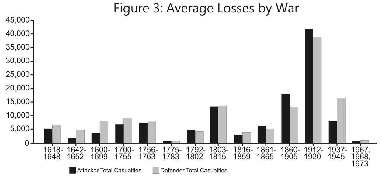
Average loses by war (see Figure 3) suffers from the same battle definition problem.

Percent losses per day (see Figure 4) is a useful comparison through the end of the 19th Century. After that, the battles get longer and the definition of a duration of the battle is up to the analyst. Note the very dear and definite downward pattern of percent loses per day from the Napoleonic Wars through the Arab-Israeli Wars. Here is a very clear indication of the effects of dispersion. It would appear that from the 1600s to the 1800s the pattern was effectively constant and level, then declines in a very systematic pattern. This partially contradicts Trevor Dupuy’s writing and graphs (see Figure 1). It does appear that after this period of decline that the percent losses per day are being set at a new, much lower plateau. Percent losses per day by war is attached.

Looking at the actual subject of the dispersion of people (measured in people per kilometer of front) remained relatively constant from 1600 through the American Civil War (see Figure 5). Trevor Dupuy defined dispersion as the number of people in a box-like area. Unfortunately, l do not know how to measure that. lean clearly identify the left and right of a unit, but it is more difficult to tell how deep it is Furthermore, density of occupation of this box is far from uniform, with a very forward bias By the same token, fire delivered into this box is also not uniform, with a very forward bias. Therefore, l am quite comfortable measuring dispersion based upon unit frontage, more so than front multiplied by depth.

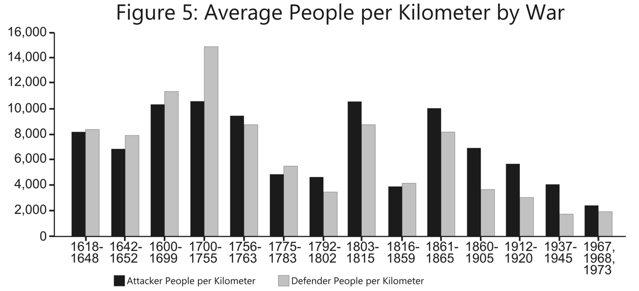Note, when comparing the Napoleonic Wars to the American Civil War that the dispersion remains about the same. Yet, if you look at the average casualties (Figure 3) and the average percent casualties per day (Figure 4), it is clear that the rate of casualty accumulation is lower in the American Civil War (this again partially contradicts Dupuy‘s writings). There is no question that with the advent of the Minié ball, allowing for rapid-fire rifled muskets, the ability to deliver accurate firepower increased.

As you will also note, the average people per linear kilometer between WWI and WWII differs by a factor of a little over 1.5 to 1. Yet the actual difference in casualties (see Figure 4) is much greater. While one can just postulate that the difference is the change in dispersion squared (basically Dupuy‘s approach), this does not seem to explain the complete difference, especially the difference between the Napoleonic Wars and the Civil War.

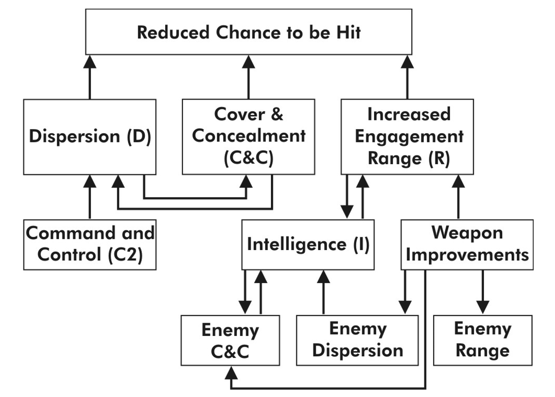
lnstead of discussing dispersion, we should be discussing “casualty reduction efforts.” This basically consists of three elements:

• Dispersion (D)
• Increased engagement ranges (R)
• More individual use of cover and concealment (C&C).

These three factors together result in the reduced chance to hit. They are also partially interrelated, as one cannot make more individual use of cover and concealment unless one is allowed to disperse. So, therefore. The need for cover and concealment increases the desire to disperse and the process of dispersing allows one to use more cover and concealment.

Command and control are integrated into this construct as being something that allows dispersion, and dispersion creates the need for better command control. Therefore, improved command and control in this construct does not operate as a force modifier, but enables a force to disperse.

Intelligence becomes more necessary as the opposing forces use cover and concealment and the ranges of engagement increase. By the same token, improved intelligence allows you to increase the range of engagement and forces the enemy to use better concealment.

This whole construct could be represented by the diagram at the top of the next page.

Now, I may have said the obvious here, but this construct is probably provable in each individual element, and the overall outcome is measurable. Each individual connection between these boxes may also be measurable.

Therefore, to measure the effects of reduced chance to hit, one would need to measure the following formula (assuming these formulae are close to being correct):

(K * ΔD) + (K * ΔC&C) + (K * ΔR) = H

(K * ΔC2) = ΔD

(K * ΔD) = ΔC&C

(K * ΔW) + (K * ΔI) = ΔR

K = a constant
Δ = the change in….. (alias “Delta”)
D = Dispersion
C&C = Cover & Concealment
R = Engagement Range
W = Weapon’s Characteristics
H = the chance to hit
C2 = Command and control
I = Intelligence or ability to observe

Also, certain actions lead to a desire for certain technological and system improvements. This includes the effect of increased dispersion leading to a need for better C2 and increased range leading to a need for better intelligence. I am not sure these are measurable.

I have also shown in the diagram how the enemy impacts upon this. There is also an interrelated mirror image of this construct for the other side.

I am focusing on this because l really want to come up with some means of measuring the effects of a “revolution in warfare.” The last 400 years of human history have given us more revolutionary inventions impacting war than we can reasonably expect to see in the next 100 years. In particular, I would like to measure the impact of increased weapon accuracy, improved intelligence, and improved C2 on combat.

For the purposes of the TNDM, I would very specifically like to work out an attrition multiplier for battles before WWII (and theoretically after WWII) based upon reduced chance to be hit (“dispersion”). For example, Dave Bongard is currently using an attrition multiplier of 4 for his WWI engagements that he is running for the battalion-level validation data base.[3] No one can point to a piece of paper saying this is the value that should be used. Dave picked this value based upon experience and familiarity with the period.

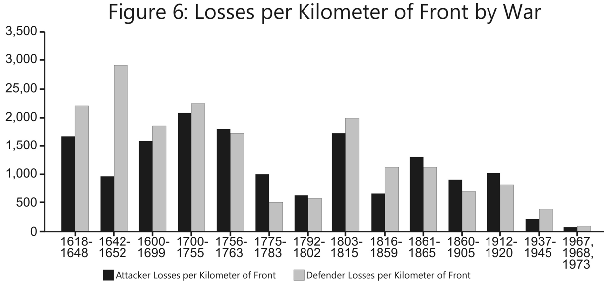
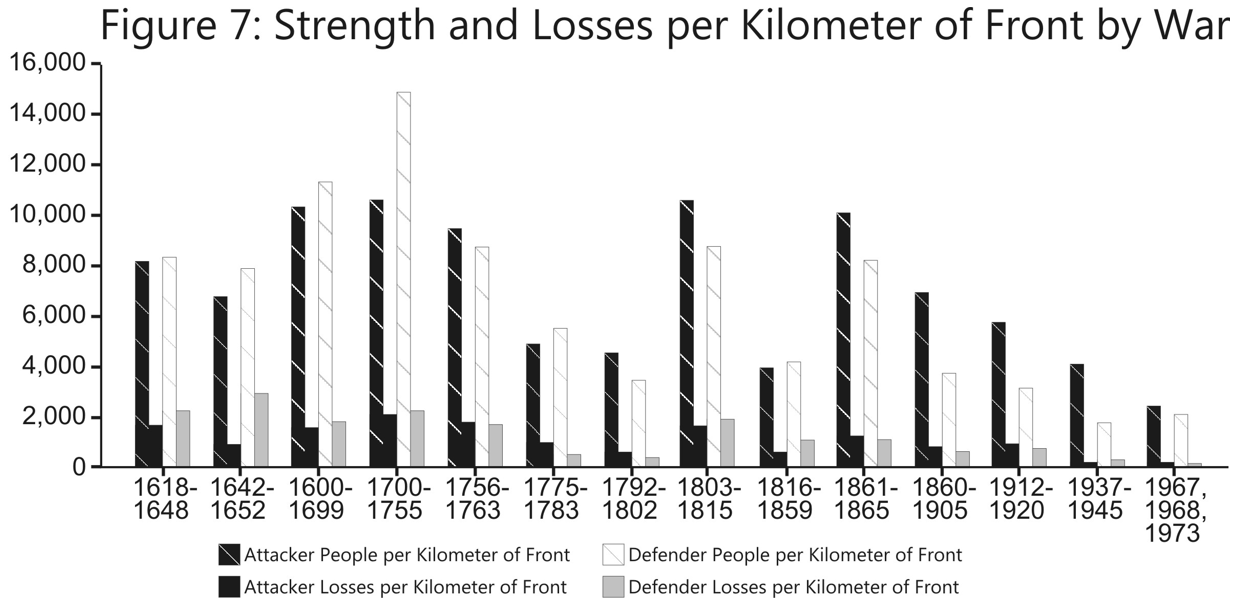I have also attached Average Loses per Kilometer of Front by War (see Figure 6 above), and a summary chart showing the two on the same chart (see figure 7 above).

The values from these charts are:

The TNDM sets WWII dispersion factor at 3,000 (which l gather translates into 30,000 men per square kilometer). The above data shows a linear dispersion per kilometer of 2,992 men, so this number parallels Dupuy‘s figures.

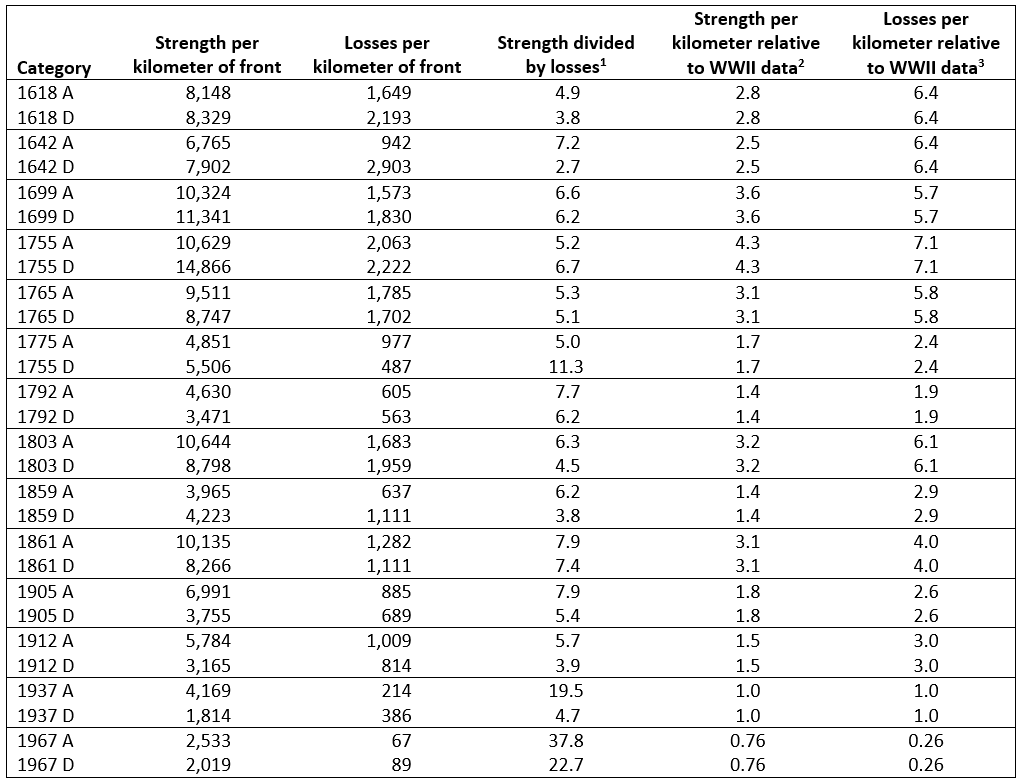
The final chart I have included is the Ratio of Strength and Losses per Kilometer of Front by War (Figure 8). Each line on the bar graph measures the average ratio of strength over casualties for either the attacker or defender. Being a ratio, unusual outcomes resulted in some really unusually high ratios. I took the liberty of taking out six

data points because they appeared unusually lop-sided. Three of these points are from the English Civil War and were way out of line with everything else. These were the three Scottish battles where you had a small group of mostly sword-armed troops defeating a “modem” army. Also, Walcourt (1689), Front Royal (1862), and Calbritto (1943) were removed. L also have included the same chart, except by century (Figure 9).
Again, one sees a consistency in results in over 300+ years of war, in this case going all the way through WWI, then sees an entirely different pattern with WWII and the Arab-Israeli Wars

A very tentative set of conclusions from all this is:

1. Dispersion has been relatively constant and driven by factors other than firepower from 1600-1815.
2. Since the Napoleonic Wars, units have increasingly dispersed (found ways to reduce their chance to be hit) in response to increased lethality of weapons.
3. As a result of this increased dispersion, casualties in a given space have declined.
4. The ratio of this decline in casualties over area have been roughly proportional to the strength over an area from 1600 through WWI. Starting with WWII, it appears that people have dispersed faster than weapons lethality, and this trend has continued.
5. In effect, people dispersed in direct relation to increased firepower from 1815 through 1920, and then after that time dispersed faster than the increase in lethality.
6. It appears that since WWII, people have gone back to dispersing (reducing their chance to be hit) at the same rate that firepower is increasing.
7. Effectively, there are four patterns of casualties in modem war:

Period 1 (1600 – 1815): Period of Stability

• Short battles
• Short frontages
• High attrition per day
• Constant dispersion
• Dispersion decreasing slightly after late 1700s
• Attrition decreasing slightly after mid-1700s.

Period 2 (1816 – 1905): Period of Adjustment

• Longer battles
• Longer frontages
• Lower attrition per day
• Increasing dispersion
• Dispersion increasing slightly faster than lethality

Period 3 (1912 – 1920): Period of Transition

• Long Battles
• Continuous Frontages
• Lower attrition per day
• Increasing dispersion
• Relative lethality per kilometer similar to past, but lower
• Dispersion increasing slightly faster than lethality

Period 4 (1937 – present): Modern Warfare

• Long Battles
• Continuous Frontages
• Low Attrition per day
• High dispersion (perhaps constant?)
• Relatively lethality per kilometer much lower than the past
• Dispersion increased much faster than lethality going into the period.
• Dispersion increased at the same rate as lethality within the period.

So the question is whether warfare of the next 50 years will see a new “period of adjustment,” where the rate of dispersion (and other factors) adjusts in direct proportion to increased lethality, or will there be a significant change in the nature of war?

Note that when l use the word “dispersion” above, l often mean “reduced chance to be hit,” which consists of dispersion, increased engagement ranges, and use of cover & concealment.

One of the reasons l wandered into this subject was to see if the TNDM can be used for predicting combat before WWII. l then spent the next few days attempting to find some correlation between dispersion and casualties. Using the data on historical dispersion provided above, l created a mathematical formulation and tested that against the actual historical data points, and could not get any type of fit.

I then locked at the length of battles over time, at one-day battles, and attempted to find a pattern. I could find none. I also looked at other permutations, but did not keep a record of my attempts. I then looked through the work done by Dean Hartley (Oakridge) with the LWDB and called Paul Davis (RAND) to see if there was anyone who had found any correlation between dispersion and casualties, and they had not noted any.

It became clear to me that if there is any such correlation, it is buried so deep in the data that it cannot be found by any casual search. I suspect that I can find a mathematical correlation between weapon lethality, reduced chance to hit (including dispersion), and casualties. This would require some improvement to the data, some systematic measure of weapons lethality, and some serious regression analysis. I unfortunately cannot pursue this at this time.

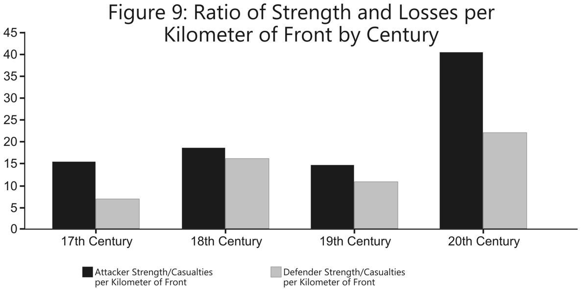
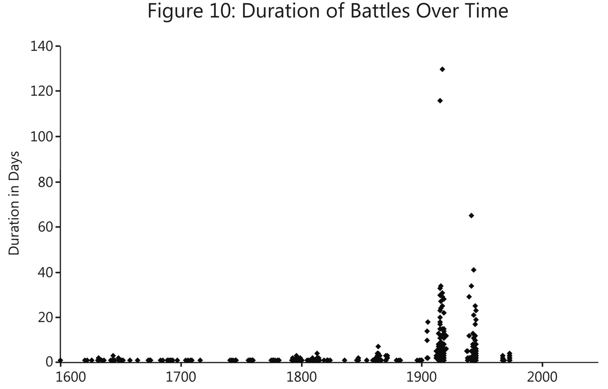
Finally, for reference, l have attached two charts showing the duration of the battles in the LWDB in days (Figure 10, Duration of Battles Over Time and Figure 11, A Count of the Duration of Battles by War).

NOTES

[1] The Tactical Numerical Deterministic Model, a combat model developed by Trevor Dupuy in 1990-1991 as the follow-up to his Quantified Judgement Model. Dr. James G. Taylor and Jose Perez also contributed to the TNDM’s development.

[2] TDI’s Land Warfare Database (LWDB) was a revised version of a database created by the Historical Evaluation Research Organization (HERO) for the then-U.S. Army Concepts and Analysis Agency (now known as the U.S. Army Center for Army Analysis (CAA)) in 1984. Since the original publication of this article, TDI expanded and revised the data into a suite of databases.

[3] This matter is discussed in Christopher A. Lawrence, “The Second Test of the TNDM Battalion-Level Validations: Predicting Casualties,” The International TNDM Newsletter, April 1997, pp. 40-50.